Fault Classification of Reciprocating Compressor Based on Neural Networks and Support Vector Machines

University of Huddersfield Repository

Ahmed, Mahmud, Abdusslam, S.A., Baqqar, Mabrouka, Gu, Fengshou and Ball, Andrew

Fault Classification of Reciprocating Compressor Based on Neural Networks and Support Vector 

Machines

Original Citation

Ahmed, Mahmud, Abdusslam, S.A., Baqqar, Mabrouka, Gu, Fengshou and Ball, Andrew (2011) 

Fault Classification of Reciprocating Compressor Based on Neural Networks and Support Vector 

Machines. In: Proceedings of the 17th International Conference on Automation & Computing. 

Chinese Automation and Computing Society, Huddersfield. ISBN 978­1­86218­098­7 

This version is available at http://eprints.hud.ac.uk/id/eprint/11491/

The University Repository is a digital collection of the research output of the

University, available on Open Access. Copyright and Moral Rights for the items

on this site are retained by the individual author and/or other copyright owners.

Users may access full items free of charge; copies of full text items generally

can be reproduced, displayed or performed and given to third parties in any

format or medium for personal research or study, educational or not­for­profit

purposes without prior permission or charge, provided:

•

The authors, title and full bibliographic details is credited in any copy;

•

A hyperlink and/or URL is included for the original metadata page; and

•

The content is not changed in any way.

For more information, including our policy and submission procedure, please

contact the Repository Team at: [email protected].

Fault Classification of Reciprocating

Compressor Based on Neural Networks and

Support Vector Machines

M. Ahmed,

S. Abdusslam

Corresponding author: [email protected]

Abstract: Reciprocating compressors play a major part in many industrial systems and faults occurring in them can degrade performance, consume additional energy, cause severe damage to the machine and possibly even system shut-down. Traditional vibration monitoring techniques have found it difficult to determine a set of effective diagnostic features due to the high complexity of the vibration signals because of the many different impact sources and wide range of practical operating conditions.

This paper focuses on the development of an advanced signal classifier for a reciprocating compressor using vibration signals. Artificial Neural Networks (ANN) and Support Vector Machines (SVM) have been applied, trained and tested for feature extraction and fault classification.

The accuracy of both techniques is compared to determine the optimum fault classifier. The results show that the model behaves well, and classification rate accuracy is up to 100% for both binary classes (a single fault present in the compressor) and multi-classes (three faults present).

Keywords: Fault Diagnosis, Reciprocating Compressor, Artificial Neural Networks, Support Vector Machine.

I. INTRODUCTION

The use of reciprocating compressors in industry has been widely reported, as has the urgent need for effective condition monitoring, which can accurately detect and diagnose the condition of the compressor see, for example [1].

The vibration signal from a reciprocating

compressor contains non-linear characteristics (e.g. due to the impacts resulting from the movement of the suction and discharge valves), and features extracted from the time, frequency and envelope domains of these signals can be used to reliably assess the health of the system. Unfortunately, not all the extracted features are equally useful in trouble-shooting, and experience has shown that even the most useful features are seldom used in the most effective way. In particular the interactions between and among features are not fully considered or even ignored [1] which may undermine the accuracy of diagnosis when the features employed are synergetic.

In this paper Support Vector Machines (SVMs) have been applied to a real compressor with single and multiple faults. It has been claimed that SVMs have four important advantages over the more traditional

ANN. First and most important, is that SVM training uses the powerful mathematical technique of global optimized solutions and so has largely eliminated a major irritant of ANNs: convergence to local maxima and minima [2]. Second the simple geometric interpretation available for SVMs has proved very useful in extending its application to new areas and theoretically can give a sparse solution – that is the solution for the lowest number of entries [3]. Third, during training, the SVM uses structural risk minimization which permits the software designer to allow for sparseness of data and which can lead to a better performance for SVMs than ANNs [4]. Fourthly, it has become clear that SVM is relatively very efficient when dealing with large classification problems (very large feature spaces), because the process of linearization means that the number of dimensions is less important with SVMs than with conventional classifiers [5]. This has the important benefit that the number of features that can be considered for fault diagnosis may be larger than could be used for ANNs.

However, it has also been pointed out that SVMs have a number of less satisfactory features: limited speed both in training and testing, extensive memory requirements, the solutions while geometrically simple can be algebraically complex, and the design of SVMs is not yet anywhere near optimal [6].

The SVM is a binary classifier it compares only two things at a time [7]. This means that if there are N items to be compared there will N*(N-1)/2 comparisons. Thus, in a real situation there will usually be will huge number of comparisons to be made. This is made worse by the parallel necessity to miss nothing of consequence when taking measurements and to ensure all possible useful features are recorded. But not all features are equally informative about the condition of the machine, and to increase the speed and accuracy of the classifier feature selection and extraction should be limited to those features useful for classification [4-5].

Comparative studies of SVMs and ANNs in fault detection with simple two-class problems (healthy or defective) found that the SVM out-performed the ANN alone in classification accuracy, while performance of the SVM and performance of the ANN combined with a Genetic Algorithm were not significantly

Proceedings of the 17

th

International Conference on

Automation & Computing, University of Huddersfield,

Huddersfield, UK, 10th September 2011

Proceedings of the 17th _{International Conference on}

0 50 100 150 200 250 300 350 400 450 500 0

0.1 0.2

(a) Envelop Spectrum at 120psi for Baseline Frequency(Hz)

A

m

p

lit

u

d

e

(V

)

0 50 100 150 200 250 300 350 400 450 500 0

0.1 0.2

(b) Envelop Spectrum at 120psi for Valve leakage Frequency(Hz)

A

m

p

lit

u

d

e

(V

)

0 50 100 150 200 250 300 350 400 450 500 0

0.1 0.2

(c) Envelop Spectrum at 120psi for Belt Looseness Frequency(Hz)

A

m

p

lit

u

d

e

(V

)

0 50 100 150 200 250 300 350 400 450 500 0

0.1 0.2

(d) Envelop Spectrum at 120psi for Inter-cooler Leakage Frequency(Hz)

A

m

p

lit

u

d

e

(V

)

different. However, it was claimed the training time for the SVM was substantially less than required by the ANN, and that the SVM was 100% successful [8].

II. VIBRATION DATA AND FEATURES

A. Datasets

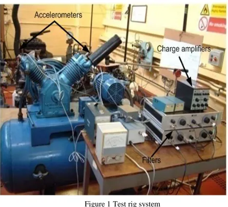
Vibration datasets were collected from accelerometers attached near the inlet and outlet valves on the first and second stage cylinder heads of a two-stage, single-acting Broom Wade TS9 reciprocating compressor. The test rig is shown in Figure 1. The compressor delivers compressed air at between 0.55 MPa and 0.8 MPa to a horizontal air receiver tank with a maximum working pressure of about 1.38 MPa. The driving motor was a three phase, squirrel cage, air cooled, type KX-C184, 2.5 kW induction motor. It was mounted on the top of the receiver tank and transfers its power to the compressor through a pulley belt system. The transmission ratio was 3.2:1, so the crank shaft speed was 440 rpm when the motor ran at its rated speed of 1420 rpm. The air in the first cylinder was compressed, passed to the higher pressure cylinder via an air cooled intercooler. When the air pressure in the storage tank reached a prescribed value, a diaphragm pressure switch switched off the electrical current to the motor. The cylinder pressures, temperatures and rotational speed were measured simultaneously with the vibration for comparison. The measured data was then fed, via a

Figure 1 Test rig system

data acquisition system to a computer for further signal conditioning and storage.

Three common faults (loose drive belt, a leaky valve in the high pressure cylinder and a leak in the intercooler) were seeded separately into the reciprocating compressor. The performance of the compressor was monitored with only one fault present at a time. Four sets of experiments were conducted one for normal operation and one for defective operation with each fault. The signal from each channel consisted of 30642

samples at a frequency of 62.5 kHz, total sampling time 0.49 seconds which is more than three working cycles of the compressor. Each data set was divided into 12 segments (bins) of 1024 samples.

B. Detection Features

The aim was to use signal processing to extract statistical features from the time, frequency and time-frequency domains which are useful for the detection and diagnosis of the seeded faults.

C. Waveform Features from Time Domain

The features extracted from the vibration signal obtained from the accelerometer on the high pressure cylinder were: root mean square (RMS), peak factor, variance, skewness, kurtosis, range, histogram lower bound (HLB), histogram upper bound (HUB) and entropy. The first five of these are well known so only the last three are defined here:

(1)

(2)

(3)

Where

and since N is the

number of samples.

D. Waveform Features from Frequency Domain

The Fast Fourier Transform (FFT) was used to transform the time-domain signal into the frequency domain from which the spectral features were obtained. The vibration spectra in Figure 2, show a number of discrete components mainly from the compressor working frequency, 7.6Hz, and its harmonics, up to 120 orders. The amplitudes vary slightly but significantly between the different faults, but it was difficult to find a simple set of features to separate the cases completely. Thus the amplitudes of these components were taken as a candidate feature, and different harmonics were used for each trial run. Thus, the resultant was a matrix of spectral features, with n harmonics and s the number of samples.

III. Probabilistic Neural Network

The PNN is a type of supervised neural network introduced by Specht in 1989 and used mainly for classification based on of Bayes optimal decision rule [9]:

(4)

where and are the probability density

functions for data classes and ; and are the prior

probabilities; and are misclassification data

classes. Thus a vector is classified into class i if the product of all the three terms is greater for data class i

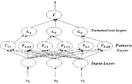
than for any other data class j not equal to i. In most applications, the prior probabilities and costs of misclassifications are treated as being equal as far as the density functions are concerned. In implementing neural network architecture, a PNN consists of an input layer, a pattern layer, a summation layer and a competitive output layer. This architecture is

illustrated in Figure 3.

Figure 3. Architecture of a PNN classifier

In recent years, PNN has been widely used in different fields such as pattern recognition and signal processing and has been recognized as a useful technique for high dimensional classification problems. In addition it also is used in CM for differentiating different faults and degrees of fault severity [10].

The PNN is considered much faster than other algorithms such as a Multi-Layer Perceptron (MLP) neural network used in [11] during the training process, which is simply to select a kernel function and its smoothing parameter when solving a linear equation set.

A. Pattern Layer

For each training cycle there is one pattern node. For classification the pattern node produces a product of the input pattern vector x with a weight vector wi such

that , (where both and are normalized)

and performs a non-linear operation on before

outputting its activation level to the summation node.

The non-linear operation is .

B. Summation Layer

The summation layer receives the outputs from the pattern layer related to a given class. It sums the inputs from the pattern layer that matched that class from which the training pattern was selected.

(5)

C. Output Layer

The output nodes have two input neurons. These units produce binary outputs, associated with two different categories using the classification principle:

( ( (6)

The outputs have only a single weight , given by the loss parameters, the prior probabilities and the number of training patterns in each category. Accordingly, the weight is the ratio ofa priori probabilities, divided by the ratio of samples, and multiplied by the ratio of

losses. These were developed using non-parametric

techniques for estimating multivariate or univariate probability density functions from random samples. The th pattern neuron in the th group computes its output using a Gaussian Kernel of the form:

(7)

Where is the centre of the kernel, and is a spread parameter which determines the size of the kernel. The summation layer of the network computes the approximation of the conditional class probability function through a combination of the previously computed densities as follows:

(8)

Where is the number of pattern neurons of class k,

and are positive coefficients

satisfying,

pattern vector

belongs to the

class that corresponds to the summation unit with

maximum output.

IV. SUPPORT VECTOR MACHINES

In describing the SVM emphasis is on the engineering and physics. If required, details of the mathematical methods can be found in, e.g.[5, 12-13].

(minimise the error bound) to give best performance. Note that this problem is linear.

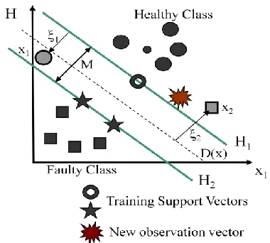
Figure 4 Classification of binary classes using SVM

In standard form the separating hyperplane must satisfy the following constraints:

yi(w·xi+ b) ≥1 i=1, 2, ..., n (9)

Where: xiis the set of training samples, w·xiis the dot

product, n is the number of samples, b is a scalar measure of the distance of H2 from the origin, and w is

the normal vector to the hyperplane. Here the samples are assumed be in only one of two classes: healthy or faulty. For the healthy class yi = +1, and faulty class, yi

= -1.

However, in most real situations such an ideal hyperplane does not exist. To find the optimum solution the standard technique is to relax the constraints on (9) by introducing a slack variable, ξi ( ≥

0). This slack variable is said to represent the noise in the system. The solution to this problem requires the application of advanced but relatively well-known

mathematical techniques. The calculation is

converted into the equivalent Lagrangian dual problem and the learning task is reduced to minimizing the primal Lagrangian with respect to w and b:

L(w, b, α) =

½||w||2 + – (10)

Where i are Lagrangian multipliers.

Finding the optimal values for i allows w to be

expressed in terms of i which allows the solution of

(10) to be found. The optimal values for i give the

decision function:

f(x) = sgn(∑ iyi ( · + b) (11)

This paper refers to a linear problem in which the training samples, and ■, were separable both in the original input space and in the feature space (hyperspace). However, with multiple dimensions, the

features in the original input space will not normally be separable. Nevertheless a suitable choice of a so-called kernel function to be used in the decision function will separate the features in hyperspace.

f(x) = sgn(∑ iyi ( )· + b) (12)

The importance of this is that the analysis performed in hyperspace becomes linear. The kernel function is written K(xi·xj) = φ(xi)φ(xj). There are now standard

kernel functions and

this paper uses

popular polynomial function [15]:

K(xi·xj) = [(xi·xj)+ 1]p. (13)

V. IMPLEMENTATION

In this work, the experiments were performed using data from the reciprocating compressor test rig, described above, and computer implementation was conducted in MATLAB.

Figure 5 shows a block flow diagram of a multi-class SVM based fault diagnosis system which consists of three sections: data acquisition, feature extraction and selection, and training and testing for fault diagnosis.

Compressor sensors-Data Acquisition

Features Extraction

Training Data Set Testing Data Set

Kernel Transform Kernel Transform

Optimal Hyperplane

Decision

Classification Result

Figure 5 Flow chart of SVM based monitoring

Baseline features were extracted to form a healthy vector feature and faulty conditions created as a vector. A target vector was created the same length as the data vectors. Both data vectors and target vector were divided into two subsets of equal size by taking every other vector value, of which one was for training the SVM and the other for testing. In this particular work a feature selection technique ranks the extracted features and the most important are used as input features. Finally, the SVMs are trained and used to classify the machinery faults.

two are for the time-domain feature based SVM, the other two is for the frequency-domain feature based SVM.

VI. RESULTS AND DISCUSSION

Table 1 presents classification results obtained for the SVMs using features extracted from the frequency-domain. There were a total of 120 peaks in the frequency spectrum and each one was a possible feature. In each table there is a column headed “number of features”, the 15 or 20 or other number of features are those which gave the best result. The table includes performance of SVM classifier with a binary class using features from the frequency-domain, and performance of the SVM classifier with multiple classes using features from the frequency-domain.

Number of input features from the frequency domain

Classification success rate %

binary class,

Classification success rate %

multiple class

15 92.36 83.33

20 85.42 72.92

30 93.75 72.92

45 93.75 82.64

50 94.44 84.03

60 88.33 73.61

75 89.56 79.86

85 84.72 74.31

100 85.45 74.31

120 86.80 71.53

Table 1 Performance of SVM classifier: features from the frequency-domain, single and multiple classes

Table 2 presents results obtained for previously in exactly corresponding situations using a PNN. A comparison shows the PNN is more successful when smaller numbers of features are used, but less

successful with larger numbers of features.

Interestingly, overall the PNN was more successful than the SVM both at detecting the presence of a single fault (leaky valve) 98.61% compared to 94.44%, and detecting the presence of the three faults, 95.83% compared to 84.03% .

Number of input features from the frequency domain

Classification success rate %

binary class,

Classification success rate % multiple class

10 84.72 81.94

15 84.72 81.94

20 91.67 87.70

30 95.83 93.75

45 95.83 93.75

50 97.92 95.14

60 98.61 95.14

65 98.61 95.83

75 88.89 84.03

80 81.25 77.78

85 79.17 72.92

100 71.53 61.81

120 68.75 51.39

Table 2 Performance of PNN classifier: features from the frequency-domain, binary and multiple classes

Table 3 present classification results for binary class fault detection obtained with the SVMs using features extracted from the time-domain. As explained and listed above, nine features were extracted and these were used in different combinations to detect the presence of a single fault (binary classifier) or three faults (multiple classifier). To avoid the need for an extra column in the tables it is stated here that the number of ways of selecting n features (1 ≤ n ≤ 9) from nine is 9Cn, e.g. there are 126 ways of selecting five

features from nine, 126 possible combinations of five features. For example, in the second row of Table 3, features are selected two at a time from the total of nine possible features, there are 36 possible ways of doing this. Of the 36 possible combinations only two (Peak factor and Kurtosis, and Peak factor and Skewness) give the highest classification rate (75%). It can be seen that the SVM was 100% successful in detecting the presence of a single fault when 4, 5, 6 and 7 features were used, but was only 100% successful in detecting the presence of three faults when 5 and 6 features were used.

Number of features used in classification

Number of combinations of features giving highest

classification rate

Highest classification success rate %

1 1 50.00

2 2 75.00

3 3 95.83

4 3 100

5 19 100

6 16 100

7 6 100

8 2 100

9 1 91.67

Table 3 Performance of SVM classifier; binary class fault detection using time-domain features

Number of features used in

classification

Number of combinations of

features giving highest classification rate

Highest classification success rate %

1 1 45.83

2 1 89.56

3 2 93.75

4 3 97.92

5 7 100

6 1 100

7 1 97.92

8 3 95.83

9 1 91.67

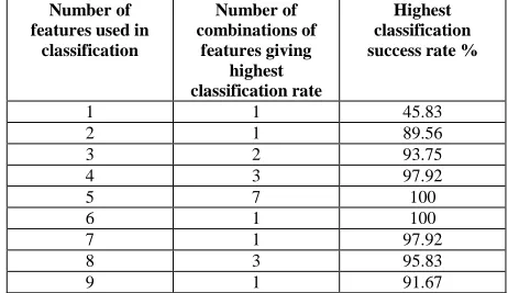
Table 4 Performance of SVM classifier; multiple class fault detection using time-domain features

Number of features used in classification

Number of combinations of features giving highest

classification rate

Highest classification success rate %

2 7 100

3 15 100

4 35 100

5 35 100

6 21 100

7 7 100

8 1 100

9 1 100

Table 5 Performance of PNN classifier; binary class fault detection using time-domain features

Number of features used in classification

Number of combinations of features giving highest

classification rate

Highest classification success rate %

1 1 65.28

2 1 80.56

3 1 93.06

4 3 91.67

5 2 91.67

6 1 91.67

7 3 88.89

8 1 88.89

9 1 83.33

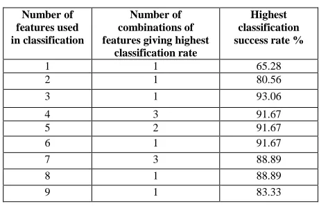
Table 6 Performance of PNN classifier; multiple class fault detection using time-domain features

The PNN classifier is generally more successful than the SVM when only one fault is present. However, the situation is reversed when diagnosing multiple faults when the SVM performed consistently better than the PNN.

VII.CONCLUSIONS

The PNN clearly performed better than the SVM when diagnosing both the single fault and the three (multiple) faults using features extracted from the frequency-domain.

The performance of the SVM improved considerably when using features extracted from the time-domain. It did not outperform the PNN in the diagnosis of a single fault (binary class) but did much better than the PNN in the diagnosis of three faults, achieving 100% when either five or six features were used.

It should be noted that use of features extracted from

the time-domain rather than frequency-domain

consistently gave a higher success rate.

REFERENCES

[1] B.-S. Yang, et al., "Condition classification of small reciprocating compressor for refrigerators using artificial neural networks and support vector machines," Mechanical Systems and Signal Processing, vol. 19, pp. 371-390, 2005.

[2] M. Rychetsky, "Algorithms and architecture for machine learning based on regularised neural

networks and support vector approaches," Sheker-Verlag, 2001.

[3] V. Vapnik, "The nature of statistical learning theory," Springer, New York, 1999.

[4] V. Ghate, Dudel, S, "Induction machine fault detection using support vector machine based classifier," WSEAS Transactions on Systems, vol. 8, pp. 591-603, 2009.

[5] A. Widodo, Yang, B-S. , "Support vector machine in condition monitoring and fault diagnosis,"

Science Direct, Mechanical Systems and Signal Processing, vol. 21, 2007.

[6] J. e. a. Suykens, "Least squares support vector machines," World Scientific Publishing Company, London, 2003.

[7] C. Wei, Chih, H., Lin, J. , "A comparison of methods for multi-class support vector machines,"

IEEE Trans. On Neural Networks, vol. 13, pp. 415-425, 2002.

[8] B. Samanta, "Gear fault detection using artificial neural networks and support vector machines with genetic algorithms," Mechanical Systems and Signal Processing, vol. 18, pp. 625-644, 2004. [9] S. P. Specht DF, "On fully automatic feature

measurement for banded chromosome classification," Cytometry, vol. 10, 1989.

[10] D. F. Specht, "Probabilistic neural networks,"

Neural Networks, vol. 3, pp. 109-118, 1990. [11] H. a. Liao, "A comparative study of feature

selection methods for probabilistic neural networks in cancer classification," Proc. 15th IEEE Internat. Conf. on Tools with Artificial Intelligence, vol. ICTAI, 2003.

[12] Z. Chen, Lian, X "Fault diagnosis for valves of compressors based on support vector machine,"

IEEE Chinese Control and Decision Conference,

pp. 1235 – 1238, 2010.

[13] S. Gunn, "Support vector machines for classification and regression," Technical Report Faculty of Engineering, Science and Mathematics, School of Electronics and Computer Science, Southampton University, 1998.

[14] H. P. Chapelle O., Vapnik V.N "Support vector machine for histogram-based image classification,"

IEEE Trans on Neural Networks, vol. 10, pp. 1055-1064, 1999.

[15] Z. Chen, Lian, X, "Fault diagnosis for valves of compressors based on support vector machine,"

IEEE Chinese Control and Decision Conference