Munich Personal RePEc Archive
Generalized Fixed-T Panel Unit Root
Tests Allowing for Structural Breaks
Karavias, Yiannis and Tzavalis, Elias
July 2012
Online at
https://mpra.ub.uni-muenchen.de/43128/
Generalized …xed-
T
Panel Unit Root Tests Allowing for
Structural Breaks
Yiannis Karavias and Elias Tzavalis*
Department of Economics
Athens University of Economics & Business
Athens 104 34, Greece
July 2012
Abstract
In this paper we suggest panel data unit root tests which allow for a structural breaks in the individual e¤ects or linear trends of panel data models. This is done under the assumption that the disturbance terms of the panel are heterogenous and serially correlated. The limiting distributions of the suggested
test statistics are derived under the assumption that the time-dimension of the panel (T) is …xed, while
the cross-section (N) grows large. Thus, they are appropriate for short panels, where T is small. The
tests consider the cases of a known and unknown date break. For the latter case, the paper gives the analytic form of the distribution of the test statistics. Monte Carlo evidence suggest that our tests have
size which is very close to its nominal level and satisfactory power in small-T panels. This is true even
for cases where the degree of serial correlation is large and negative, where single time series unit root tests are found to be critically oversized.
JEL classi…cation: C22, C23
Keywords: Panel data models; unit roots; structural breaks; *Corresponding author
1
Introduction
A vast amount of work has been recently focused on drawing inference about unit roots based on dynamic
panel data models (see, Hlouskova and Wagner (2006), for a more recent survey). Since many empirical
panel data studies rely on short panels, of particular interest is testing for a unit root in dynamic panel data
model when the time dimension of the panel, denoted as T, is …xed (…nite) and its cross-section, denoted as N, grows large (see, e.g. Blundell and Bond (1998), Harris and Tzavalis (1999, 2004), Arellano and Honore (2002) and Binder et al (2005)). These tests have better small-T sample performance, compared to
large-T panel unit root tests (see, e.g., Levin et al (2002)), given that they assume …niteT In this paper, we extend the …xed-T panel data unit roots test statistics of Harris and Tzavalis (1999, 2004) to allow for
a common structural break in the deterministic components of panel data models, namely their individual
e¤ects or linear trends of a known and unknown date. This is done in a generalized dynamic panel data
framework which allows for heterogenous and serially correlated disturbance terms, for all units of the panel.
This assumption makes the tests applicable under quite general panel data generating processes, observed
in reality. The maximum order of serial correlation allowed is a function ofT.
The extension of …xed-T panel unit root tests to allow for structural breaks is very useful given evidence
supporting the view that the presence of unit roots in economic time series can be falsely attributed to the
existence of structural breaks in their deterministic components (see, e.g., Perron (2006), for a survey). On
this front, the panel data approach o¤ers an interesting and unique perspective that it is not shared by single
time series tests. The cross-sectional dimension of the panel can provide useful information, which can help
to distinguish the type of shifts (breaks) in the deterministic components of the panel from the e¤ects of
stochastic permanent shocks. As pointed out by Bai (2010), this framework can more accurately trace out
structural break points of the panel data.1 There are a few studies in the literature which suggest …xed-T
panel data unit root tests allowing for a common structural break in the deterministic components of the
panel data model (see, more recently, Karavias and Tzavalis (2012)). These studies however suggest unit
root tests using the simple AR(1), dynamic panel data model as an auxiliary regression model, which may
not be operational in practice due to the assumption of no serial correlation in its disturbance terms. The
main goal of these studies is to pass ideas how to test for unit roots in the presence of structural breaks,
1Detecting procedures of structural breaks for stationary panel data models have been also suggested in the literature by De
considering mainly the case of a known date break point. In addition to the above, there are also studies in
the literature which suggest panel unit root tests allowing for a common structural break, but they assume
thatT is large and grows faster thanN(see, e.g., Carrion-i-Silvestre et al (2005), Bai and Carrion-i-Silvestre (2009), and Kim (2011)). These tests are appropriate for large-T panel data sets. Application of these tests
to small-T panel data sets will lead to serious size distortions and critical power reductions of them. As
shown in Karavias and Tzavalis (2012), the existence of a break in the data generating process requires panel
data sets with a quite large time-dimension, T (e.g. T >150), so as large-T panel unit root tests to have satisfactory size and power performance in short panels.
The paper suggests panel data unit root test statistics allowing for a structural break in both cases of a
known and an unknown date break. The second category of test statistics relies on a sequential application
of the …rst, such as that suggested by Zivot and Andrews (1992), Andrews (1993), Perron and Vogelsang
(1998), inter alia), for single time series. The limiting distribution of these test statistics is obtained as the minimum value of a …nite number of correlated variates; T 2 for the dynamic panel data model with individual e¤ects and T 3 for the extension of this model allowing also for individual linear trends. This distribution is derived analytically, based on recent results of Arellano-Valle and Genton (2008) who
have derived the analytic form of the probability density function of the maximum of absolutely continuous
dependent random variables. The analytic form of this distribution enables us to derive critical values of
our suggested test statistics without having to rely on Monte Carlo analysis. This substantially facilitates
application of the tests in practice and their generalization to the case of serially correlated disturbance
terms.
The paper is organized as follows. In Section 2, we derive the limiting distributions of the test statistics
under the assumption that the disturbance terms of the panel data models considered are white noise
processes. This analysis will helps us to better interpret the limiting distribution of the sequential version
of the test statistics, in the case of an unknown date break. In Section 3, we generalize the test statistics
to allow for serial correlation in the disturbance terms. In Section 4 we extend the tests to allow also for
individual linear trends. In this section, we also show how to carry out the tests when there is a break in
the individual e¤ects of panel data models under the null hypothesis of unit roots. Section 5 conducts a
Monte Carlo simulation study to examine the small sample performance of the tests. Section 6 concludes
2
Test statistics and their limiting distribution
In this section, we present panel unit root test statistics under the assumption that the disturbance terms of
the AR(1) panel data model considered are independently, identically normally distributed (N IID). This is
done, …rst, for the known date break case and, then, for the unknown. Extensions of the tests to the more
general case of serially correlated and heterogenous disturbance terms are made in the next section.
2.1
Known date break
Consider the following AR(1) nonlinear dynamic panel data model:
yit=a( )it (1 ') +'yit 1+uit; i= 1;2; ::; N, (1)
where '2( 1;1],a( )it =a(1)i if t T0 and a(2)i ift > T0, whereT0 denotes the time-point of the sample,
referred to as break-point;where a common break in the individual e¤ects of panel data model (1) i occurs,
for all cross-section units of the panel i. a(1)i and a(2)i denote the individual e¤ects of model (1) before and after the break pointT0, respectively. Throughout the paper, we will denote the fraction of the sample that
this break occurs as , i.e. = T0
T 2I= 2 T;
3 T; :::::;
T 1 T .
Under the null hypothesis of a unit root (i.e. ' = 1), model (1) reduces to the pure random walk model yit =yit 1+uit, for all i, while, under the alternative of stationarity (i.e. ' < 1), it considers a
common structural break in individual e¤ects ai. The above speci…cation of the null and the alternative
hypotheses is very common in single time series unit root inference procedures allowing for structural breaks
(see, e.g., Zivot and Andrews (1992), Andrews (1993), Perron and Vogelsang (1998). The main focus of
these procedures is to diagnose whether evidence of unit roots can be spuriously attributed to the ignorance
of structural breaks in nuisance parameters of the data generating processes like individual e¤ectsai. The
common break assumption across all units of the panel i can be attributed to a monetary regime shift, which is common across all economic units, or to a structural economic shock which is independent of the
disturbance termsuit, like a credit crunch or an exchange rate realignment. As aptly noted by Bai (2010),
even if each series of the panel data model has its own break point, the common break assumption acrossi is useful in practice not only for its computational simplicity, but also because it allows for estimating the
The AR(1) panel data model (1) can be employed to carry out unit root tests allowing for a structural
break in individual e¤ects a( )it based on the within groups least squares (LS) estimator of autoregressive coe¢cient of ', denoted as '^( ). This estimator is also known as least square dummy variable (LSDV)
estimator (see, e.g., Baltagi (1995),inter alia). Under null hypothesis'= 1, it implies:
^
'( ) 1 =
"N X
i=1
y0
i; 1Q( )yi; 1
# 1"N
X
i=1
y0
i; 1Q( )ui
#
, (2)
where yi = (yi1; :::; yiT)0 is a (T X1)-dimension vector collecting the time series observations of dependent
variable yit of each cross-section unit of the panel i, yi; 1 = (yi0; :::; yiT 1)0 is vectoryi lagged one period
back,ui = (ui1; :::; uiT)is a (T X1)-dimension vector of disturbance termsuitandQ( )is the(T XT)“within”
transformation matrix of the individual series of the panel data model,yit. Let us de…neX( ) e(1); e(2)
to be a matrix of deterministic components used by the LSDV estimator to demean the levels of seriesyit,
for all i; where e(1) and e(2) are (T X1)-column vectors whose elements are de…ned as follows: e(1) t = 1 if
t T0 and 0 otherwise, and e(2)t = 1 if t > T0 and 0 otherwise. Then, matrix Q( ) will be de…ned as
Q( )=IT X( )(X( )0X( )) 1X( )0, whereIT is an identity matrix of dimension (T XT).
Panel data unit root testing procedures based on above LSDV estimator '^( ) have the very interesting property that, under the null hypothesis of'= 1, are invariant (similar) to the initial conditions of the panel yi0and, after appropriate speci…cation of matrix X( ), to the individual e¤ects of the panel data model, as
will be seen in Section 4. The latter happens if matrixX( )also contains broken linear trends. Similarity of
the tests with respect to initial conditionsyi0does not require any mean or covariance stationarity conditions
on the panel data processesyit, as assumed by generalized method of moments (GMM), or conditional and
unconditional maximum likelihood (ML) based panel data unit root inference procedures (see, e.g., Hsiao et
al (2002) and Madsen (2008)). These conditions may be proved restrictive in practice.2 However,'^( )is an
inconsistent (asymptotic biased) estimator of', due to the within transformation of the data which wipes o¤ individual e¤ects a( )it and/or initial conditions yi0 under null hypothesis ' = 1. Thus, our suggested
panel unit root test statistics will rely on a correction of estimator '^( ) for its inconsistency (asymptotic
bias) (see, e.g., Harris and Tzavalis (1999, 2004)). To derive the limiting distribution of these tests, we make
the following assumption about the sequence of disturbance terms fuitg.
2Furthermore, the performance of the GMM estimator over the LS may detetiorates due to the inacurate estimation of the
Assumption 1: (a1)fuig constitutes a sequence of independent identically distributed (IID) (T X1)
-dimension vectors with meansE(ui) = 0and variance-autocovariance matrices i E(uiu0i) = 2uIT <+1
and nonzero, for alli. (a2)E(uityio) =E uita(1)it =E uitait(2) = 0and8i2 f1;2; :::; Ng; t2 f1;2; :::; Tg:
(a3)E u4
it <+1; E(yi04)<+1; E (a (1)
it )4 <+1; E (a (2)
it )4 <+1 and E yi02 a (1) it
2
<+1; E y2i0 a
(2) it
2
<+1:
Condition (a1) of Assumption 1 enables us to derive under null hypothesis'= 1the limiting distribution of a panel data unit root test statistic based on estimator'^( ) by applying standard asymptotic theory for
IIDprocesses, while (a2) and (a3) are simple regularity conditions under which the suggested test statistic can be proved that is consistent under alternative hypothesis ' < 1. The following theorem provides the limiting distribution of such a test statistic, based on estimator '^( ) corrected for its bias. For analytic convenience, this is done under the assumption that disturbance termsuitare also normally distributed, i.e.
uit N IID(0; 2u);for alliandt:
Theorem 1 Let uit N IID(0; 2u), then, under null hypothesis '= 1and known , we have
Z( ) Vb( ) 1=2^( )pN '^( ) ^b
( )
^( ) 1
!
d
!N(0;1) (3)
asN ! 1, where
^
b( )
^( )
^2 utr(
0
Q( ))
1 N
PN i=1y
0
i; 1Q( )yi; 1
(4)
is a consistent estimate of the asymptotic bias of '^( ) which, under the null hypothesis, is given as b( )
( ) = 2
utr( 0Q
( )
)
2
utr( 0Q( ) ), ^
2
u is a consistent estimator of variance 2u under the null hypothesis, given as ^2u =
PN i=1 y0i
( ) y i
N tr( ( )) , where is the di¤erence operator and ( ) is a (T XT)-dimension matrix having in its
main diagonal the corresponding elements of matrix 0
Q( ), and zeros elsewhere, and V( ) is a variance function given as
V( ) = 4 uF( )
0
(KT2+IT2)F( ), (5)
whereF( ) =vec(Q( ) ( )0)
; KT2 is a (T2XT2)-dimension commutation matrix andIT2 is a (T2XT2
)-dimension identity matrix.
on the tables of the standard normal distribution. Theorem 1 shows that the asymptotic bias of estimator
^
'( ) stems from the "within" transformation matrix Q( ), which induces correlation between vectors yi; 1
and ui (see, e.g. Nickel (1981)). Since disturbance terms uit are IID, the correlation between yi; 1 and
ui comes only from the main diagonal elements of the variance-autocovariance matrices of uit, de…ned by
Assumption 1 as i E(uiu0i) = 2uIT, for alli. The above bias can be estimated by the nonparametric
estimator ^b( )
^( ) and, thus, it can be subtracted from '^
( ) 1 to obtain a test statistic which is normally
distributed and is asymptotically net of nuisance parameter e¤ects. To test null hypothesis'= 1, this test statistic is based on the o¤-diagonal elements of the sample moments of variance-autocovariance matrices i
which are equal to zero, i.e. E(uituis) = 0fors6=t. This can be better seen by writing test statisticZ( ) as
1
p
N
N
X
i=1
u0
i(
0
Q( ) ( ))ui= p1
N
N
X
i=1
trh( 0
Q( ) ( ))uiu0i
i
, (6)
(see Appendix) where ( 0
Q( ) ( )) is matrix with zeros in its main diagonal due to the subtraction
of matrix ( ) from 0
Q( ), which implies that tr ( 0
Q( ) ( ))E(uiu0i) = 0, for all i.3 Matrix ( )
allows us to capture the correlation e¤ects between vectorsyi; 1 andui, which are induced by the "within"
transformation of the data through matrixQ( ) and generate the bias of LSDV estimator'^( ). Subtracting
( )from 0
Q( )enables us to adjust'^( )for this bias. The adjusted LS estimator relies on sample moments of variance-autocovariance i with zero elements, i.e. E(uituis) = 0, fors6=t. These moments are weighted
by the elements of matrix 0
Q( ) ( ). They can be consistently estimated under null hypothesis '= 1.
Writing analytically matrix 0
Q( ) ( ) can be easily seen that the elements of this matrix put more
weights to sample moments ofE(uituis), fors6=t, withsandtde…ned immediately before break point,T0.
The next theorem establishes the consistency of test statisticZ( ).
Theorem 2 Under conditions (a1)-(a3) of Assumption 1, it can be proved that
lim
N!+1P(Z
( ) < z
ajHa) = 1; 2I, (7) whereza is the critical value of standard normal distribution at signi…cance level a.
3Note that matrix ( )is used to estimate 2
u, based on estimator^2u= PN
i=1 y0i ( ) yi
2.2
Unknown break point
In this section, we relax the assumption that break point T0 is known. We propose a panel data unit root
test statistic which, under the alternative hypothesis of stationarity, assumes that T0 is unknown. As in
single time series literature (see, e.g., Zivot and Andrews (1992) and Perron and Vogelsang (1998)), we will
view the selection of the break point as the outcome of minimizing the standardized test statisticZ( ), given by Theorem 1, over all possible break fractions (or break pointsT0) of the sample, , after trimming out the
initial and …nal parts of the time series observations of the panel data. The minimum value of test statistics
Z( ), for all 2I;de…ned asz min
2I Z
( ), will give the least favorable result of null hypothesis'= 1. Let
^mindenote the break point at which the minimum value ofZ( ), over all 2I;is obtained. Then, the null
hypothesis of'= 1will be rejected if
Z(^min)< c
min, (8)
where cmin denotes the sizea left-tail critical value of the limiting distribution ofmin
2IZ
( ). The following
theorem enables us to tabulate the critical values of this distribution at any signi…cance (size) levela.
Theorem 3 Let condition (a1) of Assumption 1 hold and uit is normally distributed. Then, under null hypothesis'= 1 and unknown , we have
z min
2IZ
( ) d! min
2I
N(0; ) (9)
asN ! 1, where [ s] is the variance-covariance matrix of the test statistics Z( ), with elements s given by the following formula:
s=
F( )0
(KT2+IT2)F(s) p
F( )0(K
T2+IT2)F( ) p
F(s)0(K
T2+IT2)F(s)
, (10)
where ands denote two di¤erent fractions of the sample that the break can occur.
The result of Theorem 3 implies that critical values of the limiting distribution of the standardized test
statisticmin
2IZ
( ), denotedc
min, can be obtained from the distribution of the minimum value of a …xed number
of T 2 correlated normal variables Z( ) with covariance matrix . Since minfZ(T2); Z( 3 T):::; Z(
T 1
maxf Z(T2); Z( 3
T):::; Z(
T 1
T )g, we can use the distribution of the maximum of normal variables Z( ) to
calculate critical valuecmin for a signi…cance levela, i.e.
P( < cmin) = P( > cmin) =a. (11)
The integral function P( > cmin) = a can be calculated numerically based on the probability density
function (pdf) of . This density function has been recently derived by Arellano-Valle and Genton (2008),
for the more general case of the maximum of absolutely continuous dependent random variables of elliptically
contoured distributions. For the case of normal random variables, it is given as
f (x) =X (x; ; ; ) (xeT 3; ; ; ; ); x2R, (12)
whereeT 3is a(T 3)-column vector of unities, ( )and ( )are the pdf and cdf of the normal distribution
with arguments given as follows:
; (x) = + (x ) ; ( ; ) 1 and ; = ; 0 ; ( ; ) 1;
where = ( ... )0
and =
2 6 6 4
; ;
; ;
3 7 7
5 are respectively the vector of means and the
variance-autocovariance matrix of the(T 2)-column vectorZ which consists of random variables Z( ), for 2I, partitioned asZ= (Z( )...Z( ))0, whereZ( )is a(T-3)-column vector consisting of the remaining elements
ofZ, which exclude Z( ):
The above pdf of random variable , de…ned asf (x), is a mixture of the normal marginal densities
(x; ; ; )corresponding to all possible break fractions of the sample . These densities are weighed with
the cdf values of the(T-3)-column vectorxeT 3, given as (xeT 3; ; (x); ; ). Intuitively, the pdf
formula given by (12) sums up the probabilities that one random variable Z( ) takes its maximum value x(implying thatZ( ) takes its minimum value), while the remaining variables, collected in vector Z( ); take values smaller thanx.
The consistency of the test given by Theorem 3 follows immediately from Theorem 2, which proves
hypothesis of' <1, test statisticZ( ) converges to minus in…nity, for 2I, then so does their minimum.
3
The generalization of the test statistics for serially correlated
and heterogenous disturbance terms
The test statistics presented in the previous section can be generalized to allow for serially correlated and
heterogenous disturbance terms uit, for all i. Due to the …xed-T dimension of panel data model (1) and
the allowance for a common structural break in the individual e¤ects ( )it , the maximum order of serial
correlation, denoted as pmax, which will be considered by the generalized test statistics is a function of the
time-dimension of the panel T. This will be assumed to be the same for both sample intervals before and after break pointT0. Later on, we will give a table of values for pmax which do not depend on the location
of the break,T0. These are very useful for the application of our tests, in practice.
To derive the limiting distribution of test statistics based on estimator'^( )under the above more general
assumptions, we will make the following assumption about the sequence of the disturbance terms fuig:
Assumption 2: (b1): fuig constitutes a sequence of independent random vectors of dimension (T X1)
with means E(ui) = 0and variance-autocovariance matricesE(uiu0i) = i [ i;ts], for alli, where i;ts=
E(uituis) = 0 for s = t+pmax+ 1; :::; T and t < s: (b2): The average population covariance matrix N N1 PNi=1 iis bounded away from zero in large samples: N;tt> 0 for some 0 >0and for allN > N0;
for someN0;and for at least onet2 f1; :::; Tg:(b3): The4+ -thpopulation moments of yi,i= 1; :::; N, are
uniformly bounded. That is, for every real (T X1) vectorlsuch thatl0
l= 1;we haveE(jl0
yij4+ )< B <1,
for someB. (b4): N1
N
X
i=1
l0
V ar(vec( yi y0i))l >
0
for some 0
>0; and for allN > N1; for some N1 and
for every real(12T(T + 1)X1)vectorl with l0
l = 1. (b5): E(uityio) =E uita(1)i =E uita(2)i = 0and 8
i2 f1;2; :::; Ng; t2 f1;2; :::; Tg.
Assumption 2 enables us to derive the limiting distribution of a normalized test statistic based on'^( ) 1
by employing standard asymptotic theory under more general conditions than those of Assumption 1 (see
White (2000)), which considers the simple case thatuit N IID(0; 2u), for alli. More speci…cally, condition
(b1) allows the variance-autocovariance matrices of disturbance termsuit, i=E(uiu0i), to be heterogenous
than T. The pattern of serial correlation considered by matrices i can capture that implied by moving
average (MA) processes of uit, often assumed for many economic series (see, e.g. Schwert (1989)). It can
be also though of as approximating that implied by AR models of uit whose autocorrelation dies out after
pmax.4 This pattern will enable us to correct LSDV '^( ) for its inconsistency due to serial correlation in
uit. This can be done based on momentsE(uit pmax 1uit)which are zero, across t, since disturbance terms
uit pmax 1 anduit are assumed to be uncorrelated (see, e.g. Kruininger and Tzavalis (2002), De Wachter,
Harris and Tzavalis (2007)).
Condition (b2) quali…es application of a central limit theorem (CLT) to derive the limiting distribution of
a test statistic'^( ) 1adjusted for the inconsistency of estimator'^( ), asN ! 1, under the more general assumptions than condition (b1). More speci…cally, Condition (b2) along with condition (b4) guarantees
that, the variance and the suggested test statistic will be di¤erent than zero. Finally, conditions (b5) and
(b3) constitute weak conditions under which the consistency of the tests can be proved. These two conditions
correspond to conditions (a2) and (a3) of Assumption 1.
Under the conditions of Assumption 2, the next theorem derives the limiting distribution of a normalized
test statistic based on estimator'^( )corrected for its inconsistency under'= 1and for a known date break point.
Theorem 4 Let conditions (b1) - (b5) of Assumption 2 hold. Then, under null hypothesis ' = 1 and known, we have
Z1( ) V^1( ) 1=2^( )1 pN '^( ) ^b
( ) 1
^( ) 1
1
!
d
!N(0;1) (13)
asN ! 1, where
^
b( )1
^( ) 1
= tr(
( ) 1 ^N) 1
N
PN i=1y
0
i; 1Q( )yi; 1
(14)
is a consistent estimate of the asymptotic bias of '^( ) which, under the null hypothesis, is given as
b( )1
( ) 1
= tr(
0
Q( ) N)
tr( 0Q( ) N)
; (15)
where matrix ( )1 is a (T XT)-dimension matrix having in its main diagonal, and itsp-lower andp upper diagonals of the main diagonal the corresponding elements of matrix 0
Q( ), and zero otherwise, ^N=
4In single time series literature,p
1 N
PN
i=1( yi y
0
i)is a consistent estimator of population variance-autocovariance matrix N and V1( ) is a variance function given as
V1( ) =F1( )0 F1( )0; (16)
where F1( ) = vec(Q( ) ( )1 0) and = 1 N
XN
i=1V ar(vec(uiu
0
i)) is the variance-covariance matrix of
vec(uiu0i).
To implement the test statistic given by Theorem 4, Z1( ), we need consistent estimates of the variance-covariance matrix of vectorvec(uiu0i), de…ned as . This can be done under null hypothesis'= 1based on
the following estimator:
^ = 1
N
N
X
i=1
(vec( yi yi0)vec( yi y0i)
0
). (17)
As ( ) forZ( ), matrix ( )
1 plays a crucial role in constructing test statisticZ ( )
1 . It adjusts LS estimator
^
'( ) for its asymptotic bias. This bias now comes from two sources: the "within" transformation of the data through matrixQ( ), which has been examined before, and the serial correlation of disturbance terms
uit.5 Subtracting ( )1 from
0
Q( ) enables to adjust'^( ) for the above two sources of bias. The adjusted
LS estimator'^( ) enables us to test the null hypothesis of'= 1 based on sample moments of the elements
of variance-autocovariance matrices i, for all i, which are mot serially correlated, i.e. E(uituis) = 0; for
s=t+pmax+ 1; :::; T andt < s. These moments are weighted by elements of matrix 0Q( ) ( )1 . These
assign higher weights to the moments which are immediately before the break pointT0than those which are
away from it. They can be consistently estimated under the null hypothesis through the variance-covariance
estimator ^. The weights that matrix 0
Q( ) ( )
1 assigns to the above elements of variance-autocovariance
matrices iobviously depend on the break point and the maximum order of serial correlationpmaxconsidered
by test statisticZ1( ). Based on the speci…cation of this matrix, Table 1 and following relationship
pmax=
T
2 2 ; (18)
where[:] denotes the greatest integer function, give values ofpmaxwhich enable us to implement test statistic
Z1( ) independently of the location of the breakT0, or sample fraction . These values are chosen so as the
5Note that, under conditions of Assumption 1, test statisticZ( )
elements of matrix 0
Q( ) ( )
1 do not assign weights to zero elements of i, which result in a zero value of
variance functionV1( ). They are useful in choosing the maximum order of serial correlationpmaxconsidered
by test statisticZ1( ), in practice, especially when the break is of an unknown date.
Table 1: Maximum order of serial correlation
T 5 6 7 8 9 10 11 12 13 14 15 16 17 18 19 20
pmax 1 1 2 2 3 3 4 4 5 5 6 6 7 7 8 8
Note that, in the case that disturbance tests uit are normally distributed, variance function V1( ) can be
written in a more analytic form as
V1( ) =F1( )0(KT2+IT2)( N N)F1( ), (19)
where denotes the Kronecker product.6 This form ofV( )
1 can be easily calculated by replacing N with
its consistent estimate ^N = N1 Pi=1N ( yi y0i).
Test statisticZ1( ) can be easily extended to the case of an unknown break point date, which requires a sequential application of it. De…ne this test statistic as z1 min
2IZ ( )
1 . Following analogous steps to those
for sequential test statisticz, it can be proved that the limiting distribution ofz1is given as
z1 min
2IZ ( ) 1
d
! 1 min
2I
N(0; 1), (20)
N ! 1, where 1 [ 1; s] is the variance-covariance matrix of the test statistics Z1( ) whose elements,
de…ned as 1; s, are given by the following formula:
1; s=
F1( )0 F (s) 1
q
F1( )0 F ( ) 1
q
F1(s)0 F (s) 1
. (21)
Critical values of the distribution of random variable 1, denoted asf 1(x1)wherex12R, can be calculated
by replacing the values of s in pdf formula (12) with those of 1; s, given by (21). This also requires to
6This can be easily seen using standard results of the variance of a quadratic form for normally distributed variates (see e.g.
Schott(1996)), which imply
obtain consistent estimates of variance-covariance matrix , in the …rst step.
4
Extension of the tests to the case of deterministic trends
In this Section, we will extend the tests presented in the previous section to allow for individual linear
trends in the panel data generating processes, referred to as incidental trends. We will consider two cases of
AR(1) panel data models with linear trends. In the …rst case, we will assume that these trends are present
only under the alternative hypothesis of stationarity (see, e.g., Karavias and Tzavalis (2012), and Zivot and
Andews (1992) for single time series), while in the second that they are present under the null hypothesis of
'= 1either (see, e.g., Kim (2011). The …rst of the above cases is more appropriate in distinguishing between nonstationary panel data series which exhibit persistent random deviations from linear trends, implied by
the presence of individual e¤ects under'= 1, and stationary panel data series allowing for broken individual linear trends under' < 1. The second case is more suitable when considering more explosive panel data series under ' = 1, which can exhibit both deterministic and random persistent shifts from their linear trends.
4.1
Broken trends under the alternative hypothesis of stationarity
Consider the following extension of the nonlinear AR(1) model (1):
yit= ( )it (1 ') +' i+ ( )
it (1 ')t+'yit 1+uit; i= 1; :::; N (22)
where ( )it are de…ned by equation (1) and ( ) it =
(1)
i ift T0 and (2)i ift > T0. Under null hypothesis
'= 1, i constitute individual e¤ects of the panel data model, which capture linear trends in the level of
series yit, for all i. Under alternative hypothesis ' < 1, i are de…ned as i = (1)
i if t T0 and (2)i if
t > T0. That is, they constitute the slope coe¢cients of individual linear trendst, for alli.
Let us de…ne matrix X( ) = (e(1); e(2); (1); (2)), where (1) and (2) are (T X1)-column vectors whose
elements are given as (1)t =t if t T0; and zero otherwise, and (2)t =t if t > T0, and zero otherwise.
Then, the "within" transformation matrix now will be written asQ( )=IT X( )(X( )
0
X( )) 1X( )0
and
^
'( ) 1 =
"N X
i=1
y0
i; 1Q ( )
yi; 1
# 1"N
X
i=1
y0
i; 1Q ( )
ui
#
. (23)
Following analogous steps to those for the derivation of test statisticsZ( )andZ( )
1 , inference about unit roots
can be conducted based on estimator'^( ) adjusted for its inconsistency. Under conditions of Assumption 2, this inconsistency is given as
b( )2 ( ) 2
= tr(
0
Q( ) N)
tr( 0Q( )
N)
(24)
(see Appendix, proof of Theorem 5). However, in contrast to the case of model (1), the average
pop-ulation variance-autocovariance matrix N can not be consistently estimated based on estimator ^N = 1
N
PN
i=1( yi y
0
i), due to the presence of individual e¤ects i under null hypothesis'= 1. It can be easily
seen that, under'= 1, yi =ui+ ie, where eis a (T X1)-vector of unities, and thus
1
N
N
X
i=1
E( yi yi0) = N + 2NJT; (25)
where JT is a T T matrix of ones and 2N = N1
PN
i=1E(( i)2): The last relationship clearly shows that
in order to provide consistent estimates of matrix N based on estimator ^N = N1 PNi=1( yi y0i), we need
to substitute out the average of squared individual e¤ects 2N entering this estimator. This can be done
with the help of a (T XT)-dimension selection matrix M, de…ned as follows: M has elements mts = 0 if
ts6= 0and mts = 1if ts= 0. That is, the elements ofM correspond to those of matrix N + 2NJT (or 1
N
PN
i=1E( yi yi0)which contain only 2
N. Based on matrixM, which implies sincetr(M N) = 0, we can
derive a consistent estimator of 2N under null hypothesis '= 1, given as
1
tr(M JT)N N
X
i=1
y0
iM yi p
! 2N, (26)
where " p!"signi…es convergence in probability. Given this estimator, we can derive a consistent estimator of the inconsistency of the LSDV estimator'^( ) for model (22), de…ned as b
( ) 2 ( ) 2 , as ^
b( )2
^( ) 2
= tr(
( ) 2 ^N) 1
N
PN i=1y
0
i; 1Q ( )
yi; 1
where ( )2 = ( ) 1 +
tr( 0Q( )
M)
trace(M JT)M (see Appendix, proof of Theorem 5),
( )
1 is a (T XT)-dimension matrix
having in its main diagonal, and itsp-lower andp upper diagonals of the main diagonal the corresponding elements of matrix 0
Q( ), and zero otherwise. It can be easily seen thattr( ( )2 ^N)constitutes a consistent
estimator of^b( )2 , sincetr( ( )2 ( N + (1)N JT)) =tr( ( )2 N).
Having derived a consistent estimator of the asymptotic bias of LS estimator'^( ) under null hypothesis '= 1net of the individual e¤ects i, next we derive the limiting distribution of a normalized test statistic
based on this estimator adjusted for its inconsistency. This is done after trimming out two time series
observations from the end of the sample, i.e. = T0
T 2 I = 2 T;
2 T; :::::;
T 2
T , due to the presence of
individual e¤ects and linear trends under alternative hypothesis of'= 1. To derive this limiting distribution and to prove the consistency of the suggest test statistic, we rely the following assumption.
Assumption 3: Let all conditions of Assumption 2 hold and we also have: E(uit i) = 0; 8 i 2
f1;2; :::; Ng; t2 f1;2; :::; Tg; E(a( )it ( )it ) = 0;8 i2 f1;2; :::; Ng.
Theorem 5 Let the sequence fyi;tg be generated according to model (22) and conditions (b1)-(b4) of As-sumption 2 hold. Then, under the null hypothesis'= 1 and known, we have
Z2( ) V^2( ) 0:5^2( )pN '^( ) 1 ^b
( ) 2
^( ) 2
!
d
!N(0;1), (28)
asN ! 1, whereV2( )=F2( )0 F2( ); is de…ned in Theorem 4, and F2( ) =vec(Q( ) ( )2 0).
Apart from the initial conditions of the panelyi0, the test statistic given by Theorem 5, de…nedZ2( ), is
similar under null hypothesis'= 1to individual e¤ects of the panel i, due to the allowance of broken trends
in the "within" transformation matrix,Q( ). To test the null hypothesis of unit roots, test statisticZ2( )relies on the same moments to those assumed by statisticZ1( ), namely E(uituis) = 0; fors=t+pmax+ 1; :::; T
and t < s. These moments now are weighted by elements of matrix 0
Q( ) ( )2 , where matrix ( )2 is appropriately adjusted to wipe o¤ the e¤ects of nuisance parameters i on the limiting distribution of the
test statistic. The maximum order of serial correlation of variance-autocovariance matrices i assumed by
test statisticZ2( ) is the same to that assumed by test statisticZ ( ) 1 .
(20), respectively. This version of the test statistic is de…ned as z2 min
2I Z ( )
2 : Its limiting distribution is
given as
z2 min
2I Z ( ) 2
d
! 2 min
2I
N(0; 2), (29)
asN ! 1, where 2 [ 2; s]is the variance-covariance matrix of test statisticsZ2( ) whose elements 2; s
are given by the following formula: 2; s= F
( )0
2 F
(s) 2
q
F( )0
2 F
( ) 2
q
F(s)0
2 F
(s) 2
: Critical values of the distribution of 2
can be derived based on pdff (x), given by (12), following analogous steps to those for test statisticz1.
4.2
Broken trends under the null hypothesis of unit roots
To allow for a common break in the individual e¤ects of the panel data model under the null hypothesis of
'= 1, consider the following extension ofAR(1)model (1):
yit= ( )it (1 ') +' ( ) it +
( )
it (1 ')t+'yit 1+uit; i= 1; :::; N (30)
Using vector notation, this model implies that, under hypothesis ' = 1, the …rst-di¤erence of vector yi is
given as yi= (1)i e(1)+ (2)
i e(2)+ui. As for model (22), this means that estimator ^N =N1 PNi=1( yi yi0)
will not lead to consistent estimates of the average population variance-autocovariance matrix N, due to
the presence of individual e¤ects (1)i and (2)i . These imply
1
N
N
X
i=1
E( yi yi0) = (1) N e
(1)
e(1)0
+ (2)N e(2)e(2)0
+ N, (31)
where J1 =e(1)e(1)0 and J2 = e(2)e(2)0. The allowance of a break in incidental parameters i under null
hypothesis'= 1requires estimation of squared individual e¤ects (1)N and (2)
N in order to obtain consistent
estimates of matrix N, net of these e¤ects. To this end, we will adopt an analogous procedure to that
following in the previous subsection, based on selection matrixM. We will de…ne two (T XT)-dimension block diagonal selection matricesM(1) andM(2), which select square individual e¤ects (1)N and (2)N , respectively. The elements of matrixM(1)are de…ned asm(1)ts = 0if ts6= 0, andm
(1)
ts = 1if ts= 0. That is, matrixM(1)
selects the elements of matrix (1)N e(1)e(1)0
+ (2)N e(2)e(2)0
+ N consisting only of e¤ects (1)N , fort; s T0.
Fort ors > T0, all elements ofM(1) are set tom(1)ts = 0. On the other hand, the elements of matrixM(2)
(1) N e(1)e(1)
0
+ (2)N e(2)e(2)0
+ N consisting only of e¤ects (2)N ;fort; s > T0. Fortors T0, all the elements
ofM(2) are set tom(2) ts = 0.
Based on the above de…nitions of matrices M(1) and M(2), we can obtain the following two consistent estimators of (1)N and (2)N :
1
tr(M(1)J 1)N
N
X
i=1
y0
iM(1) yi p
! (1)N and
1
tr(M(2)J 2)N
N
X
i=1
y0
iM(2) yi p
! (2)N , (32)
respectively, sincetr(M(j)
N) = 0forj= 1;2andtr(M(j)Jr) = 0forj; r= 1;2andj6=r. These estimators
can be employed to obtain consistent estimates of matrix N, which are net of square individual e¤ects (1)N
and (2)N . Then, a consistent estimator of the bias of the LSDV estimator '^ ( )
for model (30), de…ned as
b( )3 ( ) 3
, can be obtained as
^
b( )3
^( ) 3
= tr(
( ) 3 ^N) 1
N
PN i=1y
0
i; 1Q ( )
yi; 1
, (33)
where ( )3 = ( ) 1 +
tr( 0Q( )M(1))
trace(M(1)J1)M(1)+
tr( 0Q( )M(2))
trace(M(2)J2)M(2). Adjusting'^
( )
by the above estimator of its
bias will lead to a panel unit root test statistic whose limiting distribution is be net of squared individual
e¤ects (1)N and (2)N , under null hypothesis'= 1. In the next theorem, we derive the limiting distribution of this test statistic under the assumption of a known date break. If break pointT0is unknown, then this test
statistic will rely on a consistent estimate ofT0, in a …rst step. This can be done based on the …rst di¤erences
of the individual panel data series yit under null hypothesis'= 1, i.e. yi = (1)i e(1)+ (2)
i e(2)+ui. As
shown by Bai (2010), this estimator provides consistent estimates ofT0, which converges ato(
p
N)rate.
Theorem 6 Let the sequence fyi;tg be generated according to model (30) and conditions (b1)-(b4) of As-sumption 2 hold. Then, under the null hypothesis'= 1 and known, we have
Z3( ) V^3( ) 0:5^3( )pN '^( ) 1 ^b
( ) 3 ^( ) 3 ! d
!N(0;1), (34)
asN ! 1, where
V3( )=F ( )0
3 F ( )
3 (35)
AsZ2( ), the test statistic given by Theorem 6,Z3( ), is similar under null hypothesis'= 1to individual e¤ects (1)i and
(2)
i , due to the inclusion of broken trends in the "within" transformation matrixQ ( )
. Due
to the presence of a break under'= 1, the maximum order of serial correlation of the disturbance terms uit,pmax, allowed by statisticZ3( ) is not given by Table 1. This is given as7
pmax=
8 > > < > > :
T
2 3, ifT is even andT0= T 2
minfT0 2; T T0 2g in all other cases ofT orT0
(36)
Based on conditions of Assumption 3, it can be proved that test statistic Z3( ) is consistent, following analogous steps to those for the proof of the consistency of test statisticZ2( ). The test is also consistent, if the break point is unknown and is estimated, in the …rst step, based on the procedure mentioned above.
5
Simulation Results
In this section, we conduct a Monte Carlo study to investigate the small sample performance of the test
statistics suggested in the previous sections. For reasons of space, in our study, we consider only the case
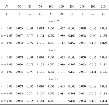
that the break date is unknown.8 We consider experiments of di¤erent sample sizes of N and T, i.e.
N =f50;100;200g and T = f6;10;15g, while the fractions of sample that the break occurs are given by the following set: = f0:25;0:5;0:75g. These value of are chosen to facilitate implementation of the test statistics. For all experiments, we conduct 10000 iterations. In each iteration, we assume that the data generating processes are given by models (1) and (22), respectively, where disturbance termsuitfollow
a MA(1) process, i.e. uit = "it+ "it 1, with "it~N IID(0;1); for all i and t, and = f 0:5;0:0;0:5g.
The values of the nuisance parameters of the simulated models, namely the individual e¤ects or the slope
coe¢cients of individual linear trends are assumed that they are driven from the following distributions:
(1)
i U( 0:5;0), (2)
i U(0;0:5); i U(0;0:05), (1)
i U(0;0:025), (2)
i U(0:025;0:05), where U( )
stands for the uniform distribution, and andyi0= 0, for alli .
7Again,p
maxis chosen so as variance functionV3( )is di¤erent than zero. IfT is even, thenpmax=minfT0 2; T T0 2g, with the exception the case thatT0=T2 wherepmax=T2 3. Consider the following examples. First,T= 10andT0= 3, then we have thatpmax= minfT0 2; T T0 2g= minf1;5g= 1. IfT0=T2 = 5, thenpmaxbecomespmax=T2 3 = 2:Note that, instead of the above, if we used the results of (18) to determinepmax, implyingpmax= minfT0 2; T T0 2g= minf3;3g= 3, thenZ3( )could not be applied sinceV3( )= 0. IfT= 15, thenpmaxbecomespmax=minfT0 2; T T0 2g. ForT0= 7;this becomespmax= minf5;6g= 5:
The small magnitude of individual e¤ects (j)i or slope coe¢cients (j)
i assumed above correspond to
evidence found in the empirical literature about them, see e.g. Hall and Mairesse (2005). The small
mag-nitude of these e¤ects makes our tests hard to distinguish null hypothesis of '= 1 from its alternative of stationarity. For all simulation experiments, we assume that the order of serial correlationpis set top= 1. This means that, for = 0, we assume an order of serial correlation which is higher than the correct order. This experiment will show if the performance of our tests critically reduces when a higher order of serial
correlation is assumed, which may happen in practice.
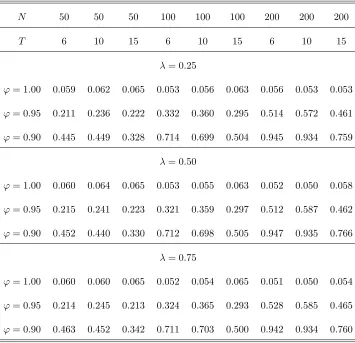
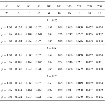
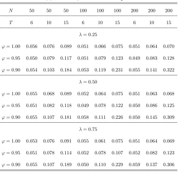
The results of our Monte Carlo analysis for test statistics z1 and z2, corresponding to models (1) and
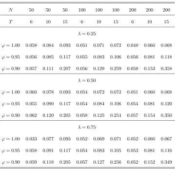
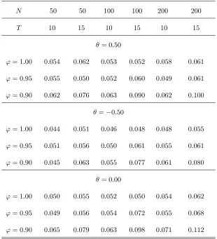
(22), are summarized in Tables 2(a)-(c) and 3(a)-(c), respectively. Table 4.presents results for test statistic
Z3( ), which is based on model (30) considering a break in individual e¤ects i under the null hypothesis. To
implement Z3( ), the break pointT0 is treated as known and it is estimated, in a …rst step. Note that this
table reports results for = 0:5andT =f10;15g, since for these cases ofT and we can assume maximum order serial correlationpmax= 1, according to equation (36). The above all tables present values of the size
and power of statisticsz1, z2 andZ3( ), for 2 f0:5; 0:5;0:0g. The size of the test statistics is calculated
for'= 1:00, while the power for'2 f0:95;0:90g. Note that, in all experiments, the power is calculated at the nominal 5% signi…cance level of the distribution of the tests.
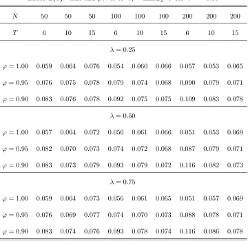
The results of Tables 2(a)-(c), 3(a)-(c) and 4 indicate that the test statistics examined, namely z1, z2
and Z3( ), have size which is close to the nominal level 5% considered. This is true for all combinations of N and T considered. The size performance of all three test statistics is close to its nominal level. This is true even if the MA parameter takes a large negative value, i.e. = 0:5. Note that, for this case of , single time series unit root tests are critically oversized (see, e.g., Schwert (1989)). The size of the test
statistics improves as N increases relative toT. This can be attributed to the fact that, as N increases relative toT, variance-covariance matrix is more precisely estimated by estimator ^. The above results hold independently on the break fraction of the sample . As a …nal note that the size of al the test statistics
does not deteriorate, if a higher order of serial correlationp= 1is assumed than the true order, for = 0. This result quali…es application of them in cases where a higher than the correct orderpof serial correlation of the disturbance termsuit is assumed in practice, i.e. p=f2;3g, which may be considered as very high
for short panels.9
Regarding the power of the test statistics, the results of the tables indicate that, as was expected, the
test statistic that has the highest power among all of them is that which corresponds to model (1), i.e. z1,
which allows for individual e¤ects under the alternative hypothesis of stationarity. For models (22) and (30),
where linear trends are considered either under alternative or null hypotheses, respectively, the power of the
test statistics (i.e., z2 and Z3( )) substantially reduces. This is feature of both single time series and panel
data unit root tests allowing for linear trends. As is well known in the literature, the second category of
tests have better power performance than the …rst (see, e.g., Harris and Tzavalis (2004), or Hluskova and
Wagner (2006)). However, between test statistics z2 andZ3( ), it is found that the …rst has clearly better
power than the second. This is true for all cases of T and N considered. The less power of statistic Z3( )
thanz2 may be attributed to the fact that this test statistic relies on estimation of the break point under
'= 1. Despite the fact that the break point is estimated very accurately under the null hypothesis, Z3( ) depends on the nuisance parameters of the sample distribution of the estimator of the break pointT0, which
may lead to a reduction of its power. Finally, note that, in contrast to the size, the power of all three test
statistics examined increases faster withT rather than N. Consistently with the theory, the power of the test statistics increases also as the value of'moves away from unity.
6
Conclusion
This paper suggests panel unit root test statistics which allow for a common structural break in the individual
e¤ects or linear trends of dynamic panel data models. Common breaks in panel data can arise in cases of
a credit crunch, an oil price shock or a change in tax policy among others. The suggested test statistics
assume that the time-dimension of the panel T is …xed (or …nite), while the cross-section N grows large. Thus, they are appropriate for short panel applications, whereT is smaller thanN. Since they are based on the least squares dummy variable (LSDV) estimator of the autoregressive coe¢cient of the dynamic
panel data model with individual e¤ects and/or linear trends, the suggested test statistics are invariant to
the initial conditions of the panel or the individual e¤ects under the null hypothesis of unit roots. This
property of the tests does not restrict their application to panel data where conditions of mean or covariance
stationarity of the initial conditions or individual e¤ects are required. To allow for serial correlation, the
tests rely on the LSDV estimator which is also corrected for its inconsistency due to a high order serial
correlation in the disturbance terms. This is done based on moments of the disturbance terms which are not
serially correlated.
The paper derives the limiting distributions of the test statistics. When the break is unknown, it shows
that the limiting distribution of the tests is calculated as the minimum of a …xed number of correlated
normals. This distribution is given, analytically, as a mixture of normals. Knowledge of the analytic
form of the limiting distribution of the tests considerably facilitates calculation of critical values for the
implementation of the tests in practice. To examine the small sample size and power performance of the
test statistics, the paper conducts a Monte Carlo study. This is done for the case that the break is of an
unknown date. The results of this exercise indicate that when there is no break under the null, the tests
have the correct nominal size and power which is bigger than their size. The size and power performance of
the test statistics does not depend on the fraction of the sample that the break occurs. As was expected, the
power of the tests is higher for the dynamic panel data models which consider individual e¤ects rather than
for the model which also allows for individual linear trends. For all cases, the power is found to increase as
N andT increases.
7
Appendix
In this appendix, we provide proofs of the theorems presented in the main text of the paper.
Proof of Theorem 1: To derive the limiting distribution of the test statistic of the theorem, we will
proceed into stages. We …rst show that the LSDV estimator '^( ) is inconsistent, as N ! 1. Then, will
construct a normalized statistic based on '^( ) corrected for its inconsistency (asymptotic bias) and derive
its limiting distribution under the null hypothesis of'= 1, as N ! 1. Decompose the vectoryi; 1for model (1) under hypothesis '= 1as
yi; 1=eyi0+ ui, (37)
Premultiplying (37) with matrixQ( ) yields
Q( )yi; 1=Q( ) ui, (38)
sinceQ( )e= (0;0; :::;0)0
. Substituting (38) into (2) yields
^
'( ) 1 =
1 N
PN i=1y
0
i; 1Q( )ui 1
N
PN i=1y
0
i; 1Q( )yi; 1
= 1 N PN i=1u 0 i 0
Q( )ui 1
N
PN i=1u
0
i 0Q( ) ui
. (39)
By Kitchin’s Weak Law of Large Numbers (KWLLN), we have
1 N N X i=1 u0 i 0
Q( )ui p
!b( )= 2utr(
0
Q( )) and 1 N N X i=1 u0 i 0
Q( ) ui p
! ( ) = 2utr(
0
Q( ) ), (40)
where " p!" signi…es convergence in probability. Using the last results, the yet non standardized statistic
Z( ) can be written by (39) as
p
N^( ) '^( ) 1 ^b
( )
^( )
!
= pN^( )
1 N
PN i=1y
0
i; 1Q( )ui
^( )
^2 utr(
0
Q( )) ^( )
!
= pN 1 N
N
X
i=1
y0
i; 1Q( )ui tr( 0Q( ))
PN i=1 y
0
i ( ) yi
N tr( ( ))
!
. (41)
Since, under the null hypothesis'= 1, we haveui= yi, (l41) can be written as follows:
p
N^( ) '^( ) 1 ^b
( )
^( )
!
= pN 1 N N X i=1 u0 i 0
Q( )ui
tr( 0
Q( ))
tr( ( ))
1 N N X i=1 u0
i ( )ui
!
= p1
N N X i=1 u0 i( 0
Q( ) ( ))ui=
1 p N N X i=1
trh( 0
Q( ) ( ))uiu0i
i
(42)
= p1
N
N
X
i=1
whereWi( ) constitute random variables with mean
E(Wi( )) = E[u0
i(
0
Q( ) ( ))ui] =tr[( 0Q( ) ( ))E(uiu0i)]
= 2utr(
0
Q( ) ( )) = 0, for alli,
sincetr( 0
Q( )) =tr( ( ))(ortr( 0
Q( ) ( )) = 0), and variance
V ar(Wi( )) = V ar(u0
i(
0
Q( ) ( ))ui) =V ar[F( )0vec(uiu0i)] =
= F( )V ar[vec(uiu0i)]F( )
0
; for alli.
The results of Theorem 1 follows by applying Lindeberg-Levy central limit theorem (CLT) to the sequence
of IID random variablesWi( ). Following standard linear algebra results (see e.g. Schott(1997), variance V ar[vec(uiu0i)] can be analytically written as V ar[vec(uiu0i)] = V ar(ui ui) = 4u(IT2 +KT2), where
denotes the Kroenecker product.
Proof of Theorem 2: Assume that the break pointT0is known. De…ne vectorw= (1; '; '2; :::; 'T 1)0
and matrix = 0 B B B B B B B B B B B B B B B B B B B B B B @
0 : : : : : 0
1 0 :
' 1 : :
'2 ' : : :
: : : : :
: : 1 0 :
'T 2 'T 3 : : ' 1 0
1 C C C C C C C C C C C C C C C C C C C C C C A
Under null hypothesis '= 1; we have = :Based on the above de…nitions of w and , vector yi; 1
can be written as
yi; 1=wyi0+ X( ) ( )i + ui, (43)
where d( )i = (a(1)i (1 '); a(2)i (1 '))0
under alternative hypothesis' <1 as follows:
Z( ) = pNVb( ) 1=2^( ) '^( ) 1 ^b
( )
^( )
!
= pNV^( ) 1=2^( ) '+
1 N
PN i=1y
0
i; 1Q( )ui 1
N
PN i=1y
0
i; 1Q( )yi; 1
1 ^
2 utr(
0
Q( )) 1
N
PN i=1y
0
i; 1Q( )yi; 1
!
= pNV^( ) 1=2^( )(' 1) +pNV^( ) 1=2 1 N
N
X
i=1
y0
i; 1Q( )ui ^2utr(
0
Q( ))
!
(44)
= npNV^( ) 1=2^( )(' 1)o
(I)
+
(
^
V( ) 1=2p1
N
N
X
i=1
(y0
i; 1Q( )ui y
0
i ( ) yi)
)
(II)
.
Next, we will show that summand (I) diverges to 1 and summand (II) is bounded in probability. These two results imply that, asN ! 1, test statisticZ( ) converges to 1, which proves its consistency.
To prove the above results, we will use the following identities:
ui=yi 'yi 1 X( )d( )i (45)
and
yi=ui+ (' 1)yi 1+X( )d( )i , (46)
which hold under alternative hypothesis' <1.
To prove that summand (I), de…ned by (44), diverges to 1, it is su¢cient to show that plim ^( )
is Op(1) and positive, and plim ^2u = Op(1) and nonzero. The last result implies that variance function
^
V( ) = ^4 uF( )
0
(KT2 +IT2)F( ) is bounded in probability. Using equations (43), (45) and (46), it can be
seen that^( ) isOp(1)as follows:
^( ) = 1
N
N
X
i=1
y0
i; 1Q( )yi; 1=
1
N
N
X
i=1
(wyi0+ X( )d( )i + ui)0Q( )(wyi0+ X( )d( )i + ui) (47)
= 1
N
N
X
i=1
(yi02w0
Q( )w+yi0w0Q( ) X( )di( )+yi0wQ( ) ui+:::+u0i
0
Q( ) ui p
!E(yi02)w
0
Q( )w+tr(X( )0 0
Q( ) X( ) d) + 2utr(
0
Q( ) ) =Op(1),
where d=E(d( )i d ( )0
the above limit are positive, since they are either variances or quadratic forms. Based on condition a3 of
Assumption 1, we can also show that the following result also holds:
^2u =
1
tr( ( ))
1 N N X i=1 y0
i ( ) yi (48)
= 1
tr( ( ))
1
N
N
X
i=1
(ui+ (' 1)yi 1+X( )d( )i )
0 ( )(
ui+ (' 1)yi 1+X( )d( )i )
= Op(1).
This limit is a nonzero quantity, since 2
u > 0. The remaining terms entered into this limit are zero or
positive quantities.
To prove that summand(II)is bounded in probability note that, by Assumption 1, we have
1 p N N X i=1
(y0
i; 1Q( )ui y0i ( ) yi) =Op(1). (49)
See also proof of Theorem 1.
Proof of Theorem 3: The proof of this theorem follows as an extension of Theorem 1, by applying
the continuous mapping theorem to the joint limiting distribution of standardized test statisticZ( ), for all
2I. The elements of the covariance matrix between random variablesZ( ) andZ( ), for all 6= , can be derived by writing
Z( )Z( ) = pN ^
( )
p
V( )
!
^
' 1 ^b
( ) ^( ) ! p N ^ ( ) p
V( )
!
^
' 1 ^b
( ) ^( ) ! = ^ ( )^( ) p
V( )pV( )N
(N1 PNi=1Wi( ))(N1 PNi=1Wi( )) ^( )^( )
= p 1
V( )pV( )
1
N
N
X
i=1
Wi( )
N
X
i=1
Wi( ). (50)
By the de…nition of Wi( ) (see (42)) and assumption of cross-section independence between Wi( ) and Wj(m), fori6=j, we haveE(Wi( )Wj( )) = 0, fori6=j. Based on this result, we can show that
plim N!1 1 N N X i=1
Wi( )
N
X
i=1
Wi( )= plim
N!1 1 N N X i=1
E(Wi( )Wi( ))can be analytically derived as
E(Wi( )Wi( )) = E[u0
i(
0
Q( ) ( ))uiu0i(
0
Q( ) ( ))ui]
= E[F( )0
vec(uiu
0
i)vec(uiu
0
i)
0
F( )] = F( )0
E[vec(uiu0i)vec(uiu0i)
0
]F( )
= F( )0
E[vec(uiu0i)vec(uiu0i)
0
]F( ), (52)
or
E(Wi( )Wi( )) = 4uF( )
0
[(IT2+KT2) +vec(IT)vec(IT)0]F( ); (53)
using the following result:
E[vec(uiu0i)vec(uiu0i)
0
] = V ar(ui ui) +E(vec(uiu0i))E(vec(uiu0i))
0
(54)
= 4u[(IT2+KT2) +vec(IT)vec(IT)0].
Based on (53), it can be shown that the probability limit of (50) is given as
E(Z( )Z( )) (55)
= F
( )0 4
u[(IT2+KT2) +vec(IT)vec(IT)0]F( ) p
F( )0 4
u[(IT2+KT2+vec(IT)vec(IT)0]F( ) p
F( )0 4
u[(IT2+KT2) +vec(IT)vec(IT)0]F( )
= F
( )0
(IT2+KT2)F( ) p
F( )0(I
T2+KT2)F( ) p
F( )0(I
T2+KT2)F( )
;
where the result of the last row follows directly fromF( )0
vec(IT)vec(IT)0= 0:
Proof of Theorem 4: The theorem can be proved following analogous steps to those for the proof of
Theorem 1.
Theorem 1 and using the following results:
1
N
N
X
i=1
u0
i
0
Q( )ui p
!tr( 0
Q( ) N) and 1
N
N
X
i=1
u0
i
0
Q( ) ui !p tr( 0Q( ) N): (56)
Based on the de…nition of matrix ( )1 and conditions (b1) and (b2) of Assumption 2, it can be easily seen
that
E(Wi( )) =tr(( 0
Q( ) ( )1 ) N) = 0, for alli. (57)
Proof of Theorem 6: It can be proved following analogous steps to those followed for the proof of
Theorem 1. Under null hypothesis'= 1, vectoryi; 1 can be decomposed as
yi; 1=yi0e+ e i+ ui. (58)
Multiplying both sides of the last relationship byQ( ) yields
Q( )yi; 1=Q( ) ui, (59)
sinceQ( )e= 0andQ( ) e= 0. Also, note that, under'= 1, the following relationships hold:
yi=ui+e i (60)
and
Q( ) yi=Q( )ui and Q( ) yi=Q( ) ui. (61)
Using (61), the numerator and denominator of'^( ) 1become
y0
i; 1Q ( )
ui=u0i
0
Q( )ui= y0i
0
Q( ) yi and (62)
y0
i; 1Q ( )
yi; 1=u0i
0
Q( ) ui= yi0
0
Q( ) yi, (63)
^
'( ) 1 =
PN i=1y
0
i; 1Q ( )
ui
PN i=1y
0
i; 1Q ( )
yi; 1 p ! b ( ) 2 ( ) 2
= tr(
0
Q( ) N)
tr( 0Q( )
N)
. (64)
The last result holds because, as N!+1, we have
1 N N X i=1 y0
i; 1Q ( )
ui tr( 0Q( )( N + 2NJT)) p
!0, where 2N =
1
N
n
X
i=1
E(( i)2), (65)
or 1 N N X i=1 y0
i; 1Q ( )
ui tr(
0
Q( ) N) p
!0,
sincetr( 0
Q( )JT) = 0; and
1 N N X i=1 y0
i; 1Q ( )
yi; 1 tr( 0Q( ) ( N + 2NJT)) p
!0; (66)
sincetr( 0
Q( ) JT) = 0:
The remaining of the proof follows the same steps with those of the proof of Theorem 1. That is, subtract
the consistent estimator of b
( ) 2 ( ) 2
, given by (33), from'^( ) 1 and, then, apply standard asymptotic theory.
References
[1] Andrews, Donald W K, 1993. Tests for Parameter Instability and Structural Change with Unknown
Change Point. Econometrica, Econometric Society, vol. 61(4), pages 821-56, July.
[2] Arelano E. and B. Honoré (2002). Panel data models: Some recent developments, Handbook of
Econo-metrics, edited by Heckman J. and E. Leamer editors, Vol 5, North Holland.
[3] Arellano-Valle, R. B., and Genton, M. G. (2008). On the exact distribution of the maximum of absolutely
continuous dependent random variables. Statistics and Probability Letters, 78, 27-35.
[4] Bai J.(2010). Common breaks in means and variances for panel data. Journal of Econometrics 157,
78-92.
[5] Bai J. and J.L. Carrion-i-Silvestre (2009). Structural changes, common stochastic trends and unit roots
[6] Baltagi B.H. (1995). Econometric analysis of panel data, Wiley, Chichester.
[7] Blundell R. and Bond S. 1998. Initial conditions and moment restrictions in dynamic panel data models.
Journal of Econometrics, Elsevier, vol. 87(1), pages 115-143, August.
[8] Binder M., Hsiao C. and Pesaran H. (2005). Estimation and inference in short panel vector autoregression
with unit roots and cointegration. Econometric Theory, 21, 795-837.
[9] Carrion-i-Silvestre J.L., Del Barrio-Castro, and E. Lopez-Bazo (2005). Breaking the panels. An
appli-cation to real per capita GDP. Econometrics Journal, 8, 159-175.
[10] De Wachter S., Harris R.D.F., Tzavalis E. (2007). Panel unit root tests: the role of time dimension and
serial correlation. Journal of Statistical Inference and Planning, 137, 230-244.
[11] De Wachter S., and Tzavalis E. (2005). Monte Carlo comparison of model and moments selection and
classical inference approach to break detection in panel data models”, Economic Letters (2005), 88,
91-96.
[12] De Wachter S., and Tzavalis E. (2012).Detection of structural breaks in linear panel data models,
Computational Statistics & Data Analysis, 56, 3020-3034.
[13] Hall, B. H. and Mairesse J. (2005). Testing for unit roots in panel data: an exploration using real and
simulated data. In D. Andrews and J. Stock (Eds.), Identi…cation and Inference in Econometric Models:
Essays in Honor of Thomas J. Rothenberg.
[14] Han, C and Phillips P.C.B (2012). GMM estimation for dynamic panels with …xed e¤ects and strong
instruments at unity. Econometric Theory, 26, 2010, 119–151.
[15] Harris R.D.F. and Tzavalis E. (1999). Inference for unit roots in dynamic panels where the time
dimen-sion is …xed. Journal of Econometrics, 91, 201-226.
[16] Harris R.D.F and Tzavalis E. (2004). Inference for unit roots for dynamic panels in the presence of
deterministic trends: Do stock prices and dividends follow a random walk?, Econometric Reviews 23,
149-166.
[17] Hlouskova J. and Wagner M. (2006). The performance of panel unit root and stationary tests: Results
[18] Hsiao C., Pesaran H. and Tahmiscioglu K., (2002). Maximum likelihood estimation of …xed e¤ects
dynamic panel data models covering short time periods. Journal of Econometrics, Elsevier, vol. 109(1),
pages 107-150, July.
[19] Karavias Y. and Tzavalis E. (2012). Testing for unit roots in short panels allowing for structural breaks.
Computational Statistics and Data Analysis, http://dx.doi.org/10.1016/j.csda.2012.10.014.
[20] Kim, D. (2011). Estimating a common deterministic time break in large panels with cross-sectional
dependence. Journal of Econometrics, 164 (2), 310-330.
[21] Kruininger H. and Tzavalis E. (2002). Testing for unit roots in short dynamic panels with serially
correlated and heteroscedastic disturbance terms. Working Papers 459, Queen Mary, University of
London, School of Economics and Finance.
[22] Levin A., Lin C.F. and Chu C-S. J, (2002). Unit root tests in panel data: asymptotic and …nite-sample
properties. Journal of Econometrics, 108, 1-24.
[23] Madsen E. (2008). GMM Estimators and Unit Root Tests in the AR(1) Panel Data Model. unpublished.
[24] Moon, H. R., Perron B. and Phillips P.C.B. (2007). Incidental trends and the power of panel unit root
tests. Journal of Econometrics, Elsevier, vol. 141(2), pages 416-459, December.
[25] Nickell, S. (1981). Biases in Dynamic Models with Fixed E¤ects. Econometrica 49, 1417-1426.
[26] Perron P. (2006). Dealing with structural breaks. Palgrave Handbook of Econometrics, Vol. 1:
Econo-metric Theory, Mills. T and K. Patterson (eds), Palgrave MacMillan, 278-352.
[27] Perron P. and Vogelsang T. (1992). Nonstationarity and level shifts with an application to purchasing
power parity. Journal of Business and Economic Statistics, 10, 301-320.
[28] Schott J.R. (1996). Matrix Analysis for Statistics, Wiley-Interscience.
[29] Stock J.H. (1994). Unit roots, structural breaks and trends. In Handbook of Econometrics, Vol. IV,
Engle R.F. and D.L. McFadden (eds), Elsevier, Amsterdam.
[30] Schwert, G.W., (1989). Tests for unit roots:a Monte Carlo investigation. Journal of Business and