Munich Personal RePEc Archive
The Impacts of Firms’ Technology
Choice on the Gender Differences in
Wage and Time Allocation: A
Cross-Country Analysis
Shirai, Daichi and Nagamachi, Kohei and Eguchi, Naotaka
20 January 2012
Online at
https://mpra.ub.uni-muenchen.de/56666/
The Impacts of Firms’ Technology Choice on the Gender
Differences in Wage and Time Allocation:
A Cross-Country Analysis
∗Daichi Shirai†, Kohei Nagamachi‡, Naotaka Eguchi§
June 15, 2014
Abstract
This paper investigates the impacts of firm technology choice on cross-country variations in gender gaps—particularly those variations in the wages and time devoted to home production. For this purpose, we construct a general equilibrium model that includes firm technology choice and home production. The numerical results reveal that the cross-country variations in both the wage and time gender gaps are substantially affected by technology choice—which suggests the persistence of the gender gap—and that a convergence in the technology choice across countries does not imply smaller cross-country variations in all gender gap–related measures.
Keywords: appropriate technology choice, gender wage gap, home production JEL classification: E13, E24, D13, J22, J16, D58
∗We would like to thank Takahisa Dejima, Fumio Hayashi, Hideaki Hirata, Ryo Jinnai, Satoshi Kawanishi, Shotaro
Kumagai, Keiichiro Kobayashi, Tsutomu Miyagawa, Daisuke Miyakawa, Kohta Mori, Kengo Nutahara, Reo Takaku, Yosuke Takeda, Hiroshi Tsubouchi, Atsuko Ueda and Daishin Yasui for their helpful comments and suggestions. For similar contributions to our paper, we would like to thank the following: the seminar participants at the Financial
Economics Workshop; CIGS workshop; A Joint Annual Meeting of Faculty of Economics, Sophia University and Nihon University; Japanese Economic Association Annual Meeting in Hokkaido University; the 14th Macroeconomics Conference; Research Institute of Capital Formation, Development Bank of Japan and Technology and Economy
Workshop; International Conference on Computing in Economics and Finance 2013. We also acknowledge the financial support provided by the Canon Institute for Global Studies and the Institute of Comparative Economic Studies, Hosei
University. All errors and opinions are our own.
†The Canon Institute for Global Studies (CIGS). E-mail address: [email protected]
‡Graduate School of Management, Kagawa University. E-mail address: [email protected]
1
Introduction
Despite the enactment of equal pay acts, equal opportunity laws, and the progress made by females
in terms of higher-education, substantial variations remain in the gender gaps of wage rates and time spent for home production—even in developed countries. What causes these differences in both the wage and time gender gaps across countries? Is there a unique mechanism that will explain the
variations in both wage and time gender gaps?
This paper investigates the cross-country variation of the gender wage gap (hereafterwage gap)
and the home production time gap (hereafter time gap) among a sample of eight industrialized nations.1 We focus on home production hours—in contradistinction to focus on market work hours by many studies, such as Olovsson (2004), Ohanian et al. (2008), and McDaniel (2011)—because
home production is more volatile than market hours between countries. In addition, recent studies emphasize the importance of the relationship between market work and home production when
comparing cross-country differences in time usage.2 However, to our knowledge, no study has yet provided a cross-country analysis of the time gap.
Meanwhile, since the mid-to-late 20th century, an increase in the female labor supply has been observed in many countries, and this trend will likely continue. Many developed countries are promoting the participation of females in the labor market to achieve work-life balance and to
address the effects of the declining birthrate and an aging society. Changing the female relative labor supply can lead to technological and institutional change that is more appropriate to female
workers, e.g., directed technical change `a la Acemoglu (2002). If labor market institutions become equalized among countries, what happens to the wage gap and the time gap?
To answer these questions, we first construct a general equilibrium model of the gender wage gap with firms technology choice and home production of households consisting of two different marital statuses: single and couple. Firms can choose their production technologies and labor
inputs. Depending on the factor abundance and relative cost of choosing different technologies, firms’ technologies can be biased toward either males or females, which results in the wage gap.
We call these technologies “gender-biased technology”. The term “technology” in this context can be broadly interpreted to include labor market institutions, corporate culture, personnel allocation, employment regulations, and social norms that affect worker productivity.
Gender-biased technology also implicitly represents the degree of unequal treatment between male and female in an intra-firm and inter-firm labor market. Employee benefits such as parental
1These countries consist of Austria, Germany, Italy, Japan, Netherlands, Spain, the United Kingdom (U.K.), and
the United States (U.S.).
2Prescott (2004) stresses the role of cross-country differences in tax rates to explain the difference in market hours
worked between U.S. and European countries using a simple neoclassical framework without home production. Later, Rogerson (2009) subsequently reports that home production drastically changes the relationship between taxes and
leave, could be an example of technology chosen by firms that would encourage female workers
to stay working in such firms after certain life events. When the female labor supply increases or more equal treatment of the genders is realized, firms would choose female-biased technology
because it is more profitable for firms to employ abundant labor factors. However, there is some empirical evidence of unequal treatment for females even in the intra-firm context, e.g., Pfeifer
and Sohr (2009), Gupta and Rothstein (2005), and Meyersson-Milgrom et al. (2001); these studies show that a distribution across job levels for female workers is strongly biased toward lower levels, and a large part of the gender wage gap can be explained by segregating males and females in
different hierarchical levels and controlling for human capital differences. To capture these unequal treatments at the macro level, we assume unequal treatment in types of technologies that include
institutions and rules, ´a la economic growth literature. Because it is difficult to take unequal treatment variables at the macro level and there are many unobserved factors that affect the working
environment, we employ a strategy that is a standard quantitative analysis that uses the economic growth model. The total factor productivity (TFP) can capture these effects instead and explicitly include such a variable.
After constructing the model, we then calibrate the parameters such that the equilibrium matches the data under the calibrated parameters. With the exception of technology choice, the
specification of the model follows the standard model in the literature and also focuses on the plainest form to facilitate interpretation. Given the limited availability of time use data, The ad-vantages of this strategy are that we can still identify all the relevant parameters, particularly for
home production; in addition, we can still identify the impacts of firm technology choice on gender gaps, which is our main interest and is clearly defined compared with other possible sources of
gender gaps that have multiple interpretations due to our calibration strategy.
The model is an application of Caselli and Coleman’s (2006) framework to the context of the
gender gap context. The Caselli and Coleman (2006) model provides that firms can choose input-specific productivities to maximize profits, in addition to a standard choice of the levels of two production inputs, skilled and unskilled workers. As a result, the skill premium reflects the relative
abundance of skilled workers, and these authors show that an important fraction of the cross-country differences in income per worker can be explained by this technology choice. Here, we treat the
gender gaps instead of the skill premium. Specifically, firms distinguish male and female labor and choose gender-specific productivities as well as labor inputs to maximize profits.3 Therefore,
given our view that technology includes institutions, institutions are endogenous variables and
3 The assumption that firms distinguish male and female labor is supported by the previous literature, which
suggests that the elasticity of substitution between males and females in market activities ranges from two to three (Olivetti and Petrongolo, 2011). Although this result might reflect differences in the skill composition between male and female, the empirical studies discussed in the text support our modeling, i.e., firms distinguish male and female
are affected by the relative supply of each production input. We also note that there is also an
exogenous friction—introduced as the relative cost of choosing technologies—that constraints firms technology choice. For example, the relative cost is affected by the degree of a taste discrimination
and the higher quit rates of females due to childbearing. The general equilibrium approach then generates rich interactions between the wage and time gaps that are frequently neglected in the
labor economics literature.
Given this approach, we restate the previous questions as follows: What are the impacts of firm technology choice on the cross-country variation in the observed gender differences in wage and
time allocation. Are the sources of the variations the same for both the wage and time gaps? To answer these questions, we conduct counterfactual simulations that compare equilibria under
appro-priate and inapproappro-priate technology choice in which firms can and cannot choose their technology depending on their environments, respectively.
The main finding is that technology choice has considerable impacts on the cross-country varia-tions in not just the wage gap but also the time gaps of both households consisting of a single person (single households) and households consisting of one male and one female (couple households) in
the sense that the observed cross-country variation in technology can significantly affect the equi-libria of countries and therefore their gender gaps. Not surprisingly, technology choice reproduces
a non-negligible part of the observed cross-country variation in the wage gap, which is also true for the time gap of single households. However, there is a different result for the time gap for couple households. That is, for the couple time gap, technology choice contributes to a reduction in the
cross-country variation, mainly because an important part of the observed cross-country variation in the couple time gap is due to the cross-country variation in the factors related to home production,
and the effect of these variations and that of technology choice on the cross-country variation offset each other.
Two policy implications are drawn from these results: The first is that there are major difficulties in narrowing gender gaps. This difficulty arises from the fact that these gaps arise largely from technology choice; this term is broadly interpreted to include labor market institutions, corporate
culture, and social norms, which are all difficult to change dramatically. The second is that global policy coordination that aims to narrow these gender gaps by affecting firms’ technology choices,
even if they succeed in altering firms’ behavior and shrinking the differences in technology choice across countries, might not result in smaller gender gaps for all measures. Instead, while achieving
smaller gaps in the wage and time gaps of single households, such a policy is associated with a widened cross-country variation in the time gap of the couple households, i.e., in some countries, the couple time gap might shrink; however, other countries might experience a larger time gap.
There are some empirical studies that conduct an international comparison of the gender wage gap, e.g., Blau and Kahn (1992, 1995, 1996a, 1996b, 2003) and Olivetti and Petrongolo (2008,
and Kahn (1999), Nickell and Layard (1999) and Boeri (2011). Blau and Kahn also argue that
institutions have an explanatory power of cross-country differences of the wage gap. However, due to their approach based on the traditional reduced form regression, they evaluate partial equilibrium
effects. We overcome this limitation by using a general equilibrium model that is able to assess the indirect effects of changing equilibria. Another difference between our studies is that we assume
endogenous institutions that are included in total factor productivity such as the economic growth model, e.g., Jones and Romer (2010), whereas Blau and Kahn treat only the observed exogenous effects of institution, e.g., parental leave and the degree of occupational segregation by gender.
The treatments we employ can assess certain unobserved technological and institutional effects of productivities.
The structure of this paper is as follows. We first describe our model in Section 2. Then, we calibrate the model and quantify the effects of firm technology choice on the cross-country
variations in the gender wage and time gaps for a benchmark case in Section 3, which is followed by a robustness analysis in Section 4. We conclude the paper in Section 5.
2
The Model
We consider a closed economy with no capital stock.4 The economic agents consist of firms, house-holds and the government. Househouse-holds are further divided into two groups: single and couple. In
addition to the production activities of firms, home production occurs in each type of household. The government conducts an income redistribution policy only. All markets are competitive.
2.1 Firms
Competitive firms employ male labor Lm and female labor Lf, which are measured in terms of efficiency units. The production technology exhibits constant returns to scale (CRS) and is specified by a constant elasticity of substitution (CES) form:
Y = [(AmLm)σ+ (AfLf)σ]
1
σ , σ <1, (1)
where Y is the output,As is sex-slabor-augmenting technology, andσ determines the elasticity of substitution (1/(1−σ)) between male and female labor. This general form of the production function is used to account for the literature. The number of empirical studies on the elasticity of substitution
is small; however, these studies consistently suggest that the elasticity of substitution ranges from two to three (Olivetti and Petrongolo, 2011). Although this result might reflect the difference in
the gender composition of the skill level between male and female, there is yet another rationale for firms to distinguish male and female labor-even when the skill levels are equal. Certain previous studies show that a distribution across job levels for female workers is strongly biased toward the
lower level, and a large part of the gender wage gap can be explained by the segregation of males and
females in different hierarchical levels even after controlling for human capital differences (Pfeifer and Sohr, 2009; Gupta and Rothstein, 2005; Meyersson-Milgrom et al., 2001).
Similar to Caselli and Coleman (2006), the model differs from the standard model in that firms choose their own appropriate technology levels, i.e., (Am, Af):
Aωm+υAωf ≤B, (2)
where ω, υ and B are all positive parameters. B is interpreted as the inverse measure of the barrier to the world technology frontier, which means a subset of the production technologies of
the most technologically advanced country, the country with the highestB. The combination ofω
andυgoverns the curvature of the country-specific technology frontier defined by the pair (Am, Af) implied by equation (2) at equality. AsB increases or the barrier diminishes, the technology frontier expands and firms within a given country can access a wider subset of production technologies. When Am/Af equals one, then equal treatment between genders is realize in the country, and the gender wage gap is narrowed.
υcan be interpreted as the relative cost of shifting from the male to the female labor-augmenting technology choice (hereafter relative cost), which reflects all sources of the gender gap in efficiency wage rates other than relative labor abundance, Ls, of the labor of each sex s. Assume that
Lm = Lf. If υ = 1, then firms choose Am = Af, i.e., there is no gender wage gap. However, if
υ >1, i.e., the relative cost is higher, firms choose the production technology such that Am > Af, which results in a gender wage gap. One possible interpretation ofυis sex discrimination (including the “glass ceiling”).5 Lazear and Rosen (1990) note that females’ higher quit rates cost employers with respect to training and promotions into higher positions.
Formally, the firms’ profit maximization problem is represented as the following:
max
{Ls, As}s∈{m,f}
n
[(AmLm)σ+ (AfLf)σ]
1
σ −wmLm−wfLf
o
s.t. (2).
In addition to the typical marginal productivity conditions used to obtain the wage gap equation,
wmem
wfef = em
ef
µ
Am
Af
¶σµ
Lm
Lf
¶−(1−σ)
, (3)
5 Arrow (1971) criticizes exogenously specified discrimination and estimates that the free entry of firms will expel
prejudiced employers in the long run, and this decreasing trend in discrimination is estimated by Flabbi (2010).
However, we do still observe discrimination. O’Neill (2003) reports that approximately 42% of the male-female gap in median earnings in 2000 could not be explained by gender differences in schooling, experience, and job characteristics.
In addition, discrimination captured by υ includes not only the employer prejudice discussed by Arrow (1971) and Becker (1971) among others, but also the asymmetric effects of policies. Furthermore, the degree and speed of decrease in discrimination might differ across countries, which provides us a rationale for conducting a cross-country analysis
assuming a condition, ω > σ/(1−σ), for a unique interior solution to the technology choice as in Caselli and Coleman (2006),6 we also have the optimality conditions for technology choice consoli-dated as
Am
Af
=υω−1σ
µ
Lm
Lf
¶ωσ−σ
, (4)
which suggests that both endogenous and exogenous comparative advantages work in technology choice. That is, the relative sex-saugmenting productivity is determined by the relative abundance and relative cost of sex-s labor. Thus, the hourly wage gap, wmem/(wfef), depends on firms’ technology choice, Am/Af, as well as the gender gap in skilles and decreasing returns to scale, the latter of which is weakened by the technology choice as the result of the complementarity between the technology choice and labor supply under the empirically valid case, i.e., σ/(ω−σ)>0.
2.2 Households
Households are divided into single and couple households. Unlike single households, members in each couple household can cooperate with one another with respect to their time allocation, which
implies that the elasticities of labor supply are different across these two different groups in general (Jones et al., 2003). Thus, letting Ns∗ and N denote the measure of the single households of sex s
and that of the couple households, respectively, the total population Nof the economy is given by
N=Nm∗ +N∗
f + 2N, which is normalized to unity without loss of generality.7
2.2.1 Single Household
A sex-ssingle household considers home production as well as the standard consumption and time allocation problem:8
max c∗
s, g∗, h∗M,s, h∗N,s≥0
(
αs∗ln(c∗s) + (1−α∗s)(1−h
∗
M,s−h∗N,s)1−γ ∗
s −1
1−γ∗
s
)
6 Intuitively, this inequality states that the degree,ω/σ, of decreasing returns to scale in technology choice
domi-nates the degree, 1/(1−ρ), of the positive circular causation in technology choice, and there is thus no benefit from
perfect specialization, and the optimal technology choice becomes the interior solution. We verify that the inequality
actually holds given the result of our calibration.
7 In the quantitative analysis, we calibrate the measures (N, N∗
m, Nf∗) under the assumption of this household
structure such that the model can match the ratio of the aggregate labor supply of each sex. Given this calibration procedure and the fact that the real world includes households with memberships other than those specified in the
model, readers should not interpret the household consisting of a couple in the model literally. Instead, it should be simply interpreted as merely a virtual representative of household members that can cooperate with one another.
Similarly, the single households should be interpreted as those without cooperation. In what follows, however, we use the terms single and couple households for convenience.
8 The input structure of home production is the same as that in Becker (1965), who was followed by Olovsson
(2004), Ragan (2013), and Rogerson (2009), among others. For preference, we follow Gronau (1977) as in Chang and
s.t.
c∗s =Hs(gs∗, esh∗N,s) =
£
ξs∗gs∗η+ (1−ξs∗)(esh∗N,s)η
¤1η
, ξ∗s ∈(0,1), η <1, (5)
(1 +τc)g∗s ≤(1−τℓ)wsesh∗M,s+T, (6)
h∗M,s+h∗N,s ≤1,
wherec∗s is the consumption of home goods produced by means of a CRS technologyHs(gs∗, esh∗N,s) with an elasticity of substitution of 1/(1−η), having inputs that consist of market goods,g∗
s and, effective home production hours, i.e., skill es times home production hour h∗N,s.9 ξs∗ is the weight of market goods in the home production of sex-s single households. Letting h∗
M,s denote market hours and normalizing the time endowment to unity, 1−h∗M,s−h∗N,sbecomes the leisure time. τcis the consumption tax, τℓ is the labor income tax, T is the lump-sum transfer per person,ws is the wage rate of sex s, α∗s is the share parameter for consumption, and γs is the inverse of the Frisch elasticity of leisure (defined as the elasticity of leisure with respect to the wage rate holding the marginal utility of consumption constant). 10
First-order conditions (FOCs) state that marginal utility from the hours for each activity balance one another:11
α∗sH
s g Hs
1−τℓ 1 +τc
wses=α∗s HsNes
Hs ,
or H s N Hs g
= 1−ξ
∗
s
ξ∗
s
Ã
gs∗ esh∗N,s
!(1−η)
= 1−τℓ 1 +τc
ws, all s∈ {m, f}, (7)
where Hs
g ≡ ∂Hs/∂g∗s, and HsN ≡ ∂Hs/∂h∗N,s. The interpretation of the first equation above is as follows. An additional market hour increases the labor income net of labor income tax by (1−τℓ)wses, which is equivalent to (1−τℓ)/(1 +τc)wses units of market goods. Multiplying this amount by marginal productivity, theHsg of market goods in home production and marginal utility of consumption α∗s/Hs, we obtain the left hand side (LHS), the marginal utility of an additional market hour. The right hand side (RHS), the marginal utility of an additional home hour, follows
a similar reasoning.
9 The inclusion of skille
s in the labor input is consistent with the arguments by Gronau(1980, 2008) that more
educated people are better at implementing their tasks. The assumption that efficiency in the home work is propor-tional to that in market activities appears less important when investigating the time gap, which is related to the ratio of efficiencies em/ef more than to the levels themselves because the difference across sexes with respect to the
impacts of education on home productivity are not decisive (Table 7 in Gronau and Hamermesh (2008)).
10Frisch elasticity is typically derived in relation to the intertemporal labor supply elasticity in dynamic models.
Although our model is static, the Frisch elasticity of leisure in our static framework is equivalent to that in dynamic models in which the utility function specifies separate leisure and time function.
11We are assuming that the zero lower bound ofh∗
M,s does not bind, which is the case of interest given that agents
Taking the ratio of each sex results in the effective time gap:
emh∗N,m
efh∗N,f =
(
wm/[(1−ξm∗)/ξm∗]
wf/[(1−ξ∗f)/ξ∗f]
)−1−1η
g∗m g∗
f
. (8)
The ratio is decreasing in the ratio of the efficiency wage, ws, normalized by the relative weight (1−ξ∗
s)/ξs∗ of home production due to the opportunity cost and increase in the ratio of market goods gs∗ due to complementarity. The elasticity of the ratio with respect to the former is precisely the same as that between market goods and labor input in home production.
2.2.2 Couple Household
A typical couple household differs from a single household in that the budget constraint is
consoli-dated and that members in the household solve a common allocation problem:12
max
g, {cs, hM,s, hN,s,zs}s∈{m,f}≥0
X
s∈{m,f}
αsln(cs) +ℓ(1−hM,m−hN,m,1−hM,f −hN,f)
(9)
s.t.
X
s∈{m,f}
cs=H(g, emhN,m, efhN,f)
=nξgη+ (1−ξ) [zm(emhN,m)ρ+zf(efhN,f)ρ]
η ρ
o1η
, ρ <1, (10)
(1 +τc)g≤(1−τℓ)
X
s∈{m,f}
wseshM,s+ 2T, (11)
hM,s+hN,s≤1, alls∈ {m, f}, (12)
whereℓis a leisure function, which is strictly increasing, twice continuously differential and concave, and H is the home production function for which the inputs consist of market goods and the CRS composite of the time of both members with an elasticity of substitution of 1/(1−ρ). The crucial difference between the above problem and the single problem is that members of the couple
households can cooperate with one another by selecting their time allocation{hM,s, hN,s}s∈{m,f}for
given weights (zm, zf), which we callzs home production effort, or simply effort, of sexshereafter. Effort is interpreted as human capital, the way in which members in a couple household cooperate with one another, and other factors. Variables and parameters that have the same notation except for an asterisk have the same meaning as for the single households. A household with two members
receives a lump-sum transfer of 2T.
Solving the allocation problem of the home goods, i.e.,{cs}s∈{m,f}, we obtain the reduced-form
problem, of which the FOCs with respect to time allocation hold that marginal utility from hours
12In this paper, we do not introduce any strategic behavior between members in the household. The input structure
to each activity balance one another as for single households:13
Hg H
1−τℓ 1 +τc
wses= Hses
H , all s∈ {m, f},
where Hg ≡∂H/∂g and Hs ≡∂H/∂(eshN,s), and the LHS and RHS are the marginal utilities of an additional market and home hour, respectively.
Furthermore, taking the ratio of this equation for each sexsyields the effective time gap for the couple households, which is similar to that for single households:
Hm Hf
= zm
zf
µ
emhN,m
efhN,f
¶−(1−ρ)
= wm
wf
, or emhN,m
efhN,f =
µ
wm/zm
wf/zf
¶−1−1ρ
, (13)
which states that the time gap depends on not only the efficiency wage gap representing the
com-parative advantage in market activities but also on the effort gap zm/zf, i.e., the comparative advantage in the home production.
This result corresponds to (8) for single households, and the effort gapzm/zf is the counterpart of the ratio of the relative weight (1 −ξs∗)/ξs∗. However, the crucial difference appears in the elasticity of the time gap with respect to the relative efficiency wage gap. The absolute elasticity
of single households is equal to the elasticity of substitution (1/(1−η)) between market goods and the time spent for home production, whereas that of the couple households is equal to the one 1/(1−ρ) between the male and female in home production. The cooperation between members in a couple household makes the market goods g public goods, which is why the above equation has no counterpart ofg∗
m/gf∗.
2.3 Government
The government levies consumption and proportional labor income taxes on households. The col-lected revenues are then used for redistribution through the lump-sum transferT per person. Thus, the government budget constraint is
NT =N τcg+
X
s∈{m,f}
Ns∗τcgs∗+
X
s∈{m,f}
N τℓwseshM,s+
X
s∈{m,f}
Ns∗τℓwsesh∗M,s. (14)
2.4 Equilibrium
Now, we can define a competitive equilibrium of the economy. We focus on a symmetric equilibrium
in which firms choose the same technology pair, i.e., (Am, Af).
Definition. Given a tax system (τc, τℓ), a symmetric competitive equilibrium of the economy is a set of a price system (wm, wf), time allocation {h∗M,s, h∗N,s, hM,s, hN,s}s∈{m,f}, quantities
({c∗s, cs, gs∗}s∈{m,f}, g,{Ls}s∈{m,f}), technology choice {As}s∈{m,f}, and a lump-sum transferT such
that
1. given prices, households maximize their utility;
2. given prices and technology constraint, firms maximize their profit;
3. markets clear:
X
s∈{m,f}
Ns∗g∗s+N g = Y, (15)
Ls = Ns∗esh∗M,s+N eshM,s ∀s∈ {m, f}; and (16)
4. the government budget constraint (14) is satisfied.
3
Quantitative Analysis
In this section, while conducting counterfactual simulations with the model described in the previous section, we ask the following question: what are the quantitative effects of technology choice on the cross-country variations in the various gender gaps, including the hourly wage gap wmem/(wfef) and time gaph∗N,m/h∗N,f of the single households and thathN,m/hN,f of the couple households. The results reveal that technology choice has a significant impact on all the gender gaps. In addition,
the mechanisms determining the time gaps of the single and couple households are also considered to be different, which implies that the convergence in Am/Af is associated with a convergence in the single time gap h∗
N,m/h∗N,f but not in the couple time gap hN,m/hN,f.
In the following subsections, we first calibrate the model and design the simulation method, which allows us to quantify the effects of technology choice on the gender gaps. We then provide
the results and focus on the importance of technology choice in the subsections that follow. In our study, we use cross-section datasets that consist mainly of the Multinational Time Use Study
(MTUS), Survey on Time Use and Leisure Activities (Japan), and the EU KLEMS. We will discuss these datasets in Appendix A.
3.1 Calibration
In the couple households, we specify the leisure function,ℓ, in the couple households as follows:
ℓ(1−hM,m−hN,m,1−hM,f −hN,f) =
X
s∈{m,f}
(1−αs)
(1−hM,s−hN,s)1−γs−1 1−γs
, (17)
where αs ∈ (0,1) is the weight of consumption. Stated differently, we assume that within each couple household, members solve a Pareto problem with equal treatment where the actions of each member affect the partner’s utility only indirectly.
the simultaneous equations derived from the FOCs and, in some cases, by using an estimation.
Intuitively, we assume that under the calibrated parameters, the equilibrium is equivalent to the observed data.14
There are 24 parameters, each of which is categorized into one of two types of parameters: household- and firm-side parameters. The household-side parameters consist of preference{α∗
s, αs, γs}s∈{m,f},
home production ({ξs∗, zs}s∈{m,f}, ξ, η, ρ), household structure ({Ns∗}s∈{m,f}, N) in workers, skill
{es}s∈{m,f}, and tax rates (τc, τℓ). The firm-side parameters consists of the elasticity of substitution (1/(1−σ)) between males and females and the technology constraint (ω, υ, B). The results of the calibration are summarized in Tables 16 and 17.
3.2 Simulation Method
In quantifying the effects of technology choice on the cross-country variations in the gender gaps, we counterfactually assume that all countries converge to the same environment, e.g., the same
U.S.-equivalent level of parameters, and then compare competitive equilibria under the following two scenarios. In each case, to obtain a competitive equilibrium, we solve the simultaneous equations
derived from the equilibrium conditions of { Y, As,ws, Ls, hM,s, h∗M,s,hN,s,h∗N,s, cs, c∗s,gs∗,g, T }s∈{m,f} in the way that is described in Appendix C. In the first scenario, firms can optimally choose their technology (we call this case the appropriate technology choice); by assumption, there are no
cross-country variations in the gender gaps after convergence in the environment. By contrast, the second scenario assumes that firms cannot choose their optimal technology and are thus faced with
the calibrated country-specificAm/Af because of sufficiently high adjustment costs or, more broadly interpreted, because of history dependence (we call this case the inappropriate technology choice).
Specifically, (Am, Af) is determined by the country-specific result Am/Am=Am,data/Af,data of the calibration and the technology constraint (2), the latter of which has the U.S. equivalent (υ, B) for all countries. In this case, we should observe cross-country variations in the gender gaps that
arise purely due to the cross-country variations in firms’ technology choices before the change in the environments.
Thus, to the extent that the cross-country variations in the gender gaps observed in the data are reproduced by the inappropriate technology choice, we can say that the effects of technology choices on the cross-country variations in the gender gaps are substantial. More specifically, by
measuring the correlation between the data and the counterfactual under the inappropriate tech-nology choice (let Corr(CF, Data) denote the correlation)— and then by calculating the ratio of
14 Because we take the values of elasticities from previous studies, this calibration approach suggests that the
parameters except for the elasticities are computed as residuals, which is why we follow the previous studies in the specification while keeping the model as simple as possible. Even with limited availability of the time use data, this method— together with the simple model— allows us to identify the values of the parameters. The procedure is
the cross-country variance V ar(CF) of some gender gap under the inappropriate technology choice to that V ar(Data) of the corresponding data— we can quantify the impacts of technology choice on the cross-country variations in the gender gaps. IfCorr(CF, Data)<0, then technology choice itself cannot explain the observed variation, and from a different perspective the larger values of
V ar(CF)/V ar(Data) imply that the observed technology choices affected the variations in the gen-der gaps more significantly. Therefore, if bothCorr(CF, Data) andV ar(CF)/V ar(Data) are near one, it can be said that technology choice itself explains the observed variations in the gender gaps. In what follows, we call the above method of comparing the inappropriate technology choice
with the data the independent experiment of technology choice. A similar method can be applied to the other sources of the cross-country variation of the gender gaps, such as effort zs, skill es and preference (α∗s, αs). Thus, to quantify the impacts of a factor, we counterfactually assume that countries are different only in this factor and compare the associated equilibrium with the data. We
also call this experiment the independent experiment. In this case, however, to exclude the effect of technology choices, the technology choices are assumed to be exogenously given in the appropriate technology level.15
We also design another type of experiment, which we callconditional experiments of technology choice. Assuming that the environments of countries except for one or some parameters of interest
converge to the U.S. equivalent, this experiment compares the two scenarios mentioned above. Thus, a conditional experiment is a slight extension of the independent experiment, and we thus quantify the impacts of factors in the same way as in the case of the independent experiment, i.e., using
the correlation Corr(CF, DAT A) and the variance ratio V ar(CF)/V ar(Data). Intuitively, this experiment quantifies the effects of the combination of several sources of cross-country variations in
gender gaps, including (at the least) technology choice.
3.3 Wage Gap
The theoretical implications of inappropriate technology choice for the wage gap may be understood by comparing the inappropriate technology choice with appropriate technology choice, in which all
countries have the same parameter values as the U.S. and firms choose their technology optimally. Then, the inappropriate technology choice is characterized by a shift of (Am, Af) on the U.S.-equivalent technology frontier.
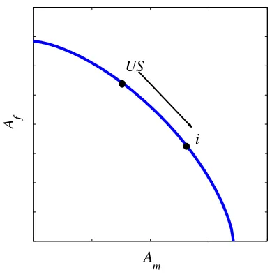
Without loss of generality, suppose that Am and Af move from a northwest point U S, which represents the U.S. or the appropriate technology choice, to a southeast point i, which represents country i on the U.S. equivalent technology frontier as illustrated in Figure 1, i.e., Am and Af increase and decrease, respectively. Because of the associated changes in labor productivities, the
15 Even assuming that the technology choice is endogenously determined, these results have a negligibly small
change from independent experiments in which the technology choice is given in the level of appropriate technology
A
m
A f
US
[image:15.612.210.405.69.269.2]i
Figure 1: Technology Shift on the U.S.-equivalent Technology Frontier
wage rate of the males and that of the females increases and decreases, respectively, which implies that the efficiency wage gap,wm/wf, increases in the manner specified by (3), all other things equal. However, this increase appears weakened by the general equilibrium effect or the associated increase in the relative aggregate labor supply of males and, therefore, its negative effect on the wage gap
due to the decreasing returns to scale. For the single household decision, the previous literature, such as Rogerson (2009), suggests that the single male (female) household increases (decreases) his (her) time spent on market activities with its response to the wage rate strengthened by substituting
between market goods and time spent on his (her) home production. For couple households, the integrated budget constraint makes the sign of the associated change in the household’s labor income
ambiguous. Thus, the magnification effects described above are now ambiguous with respect to substituting between market goods and time devoted to home production on the response of the market hour for each sex. However, even with this ambiguous magnification effect, we might expect
that an increase in the ratio hM,m/hM,f of market hours is a natural consequence of comparative advantage, which is actually the case and is confirmed by our calculations.
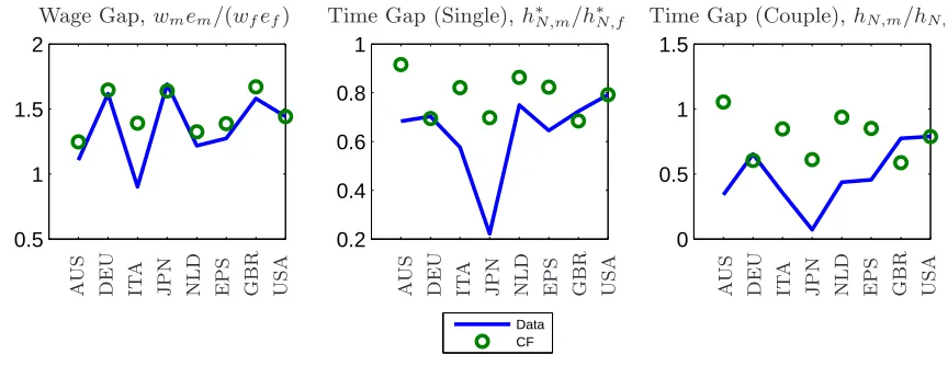
This result is then compared with the observed cross-country variation in the hourly wage gap
technology choice, respectively. The former is consistent with the literature and, together with the
latter, suggests the importance of the general equilibrium analysis that can capture the effect of the latter and verifies its relatively large impact on the cross-country variation in the wage gap.
Conditional experiments support the result of the independent experiment that technology choice is important in understanding the cross-country variation in the wage gap. Both the
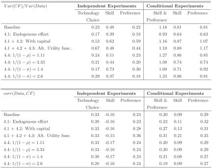
vari-ance ratio V ar(CF)/V ar(Data) and correlation Corr(Data, CF) are robust even when we add another source of the cross-country variation of the gender gaps in addition to technology choice. Importantly, the pair of technology choice and preference explains the majority of the cross-country
variation in the wage gap with a variance ratio of 0.893 and a correlation of 0.927, as indicated in Table 1; moreover, the correlation of the combination is well above the summation of the variance
ratios associated with the independent experiments of technology choice and preference. If we add either effort or skill in addition to preference, both measures move closer to one; however, compared
with the combination of technology choice and preference, the improvements are relatively small.
3.4 Single Time Gap
Suppose again that technology (Am, Af) shifts toward the southeast on the U.S. equivalent tech-nology frontier and the efficiency wage gap wm/wf thus also increases as demonstrated by the previous subsection. Each single household then takes these changes as given and chooses the time
h∗N,s devoted to her or his own home production. According to (8), the associated change in the time gap h∗
N,m/h∗N,f, is the sum of the two counteracting forces: The first is due to the associated increase in the relative opportunity costs, i.e., the change in (wm/wf)−1/(1−η), which is negative. The second is positive because of the complementarity between market goods and time devoted
to home production, i.e., the change in g∗m/g∗f which appears to increase because gm∗ (gf∗) is likely to increase (decrease) faced with an increase (decrease) in the wage rate wm (wf). The resulting change in the time gap is negative.
Then, the question is as follows to what extent can this cross-country variation in the time gap induced by technology choice explain the observed variation across countries? The independent
experiment suggests that technology choice can explain not all but some non-negligible part of of the cross-country variation in the time gaps of single households. A positive correlationCorr(Data, CF) between the data and counterfactual, although much smaller than that for of the wage gap (as
shown by the center panel of Figure 2 or Table 2), implies that the cross-country variation induced by technology choice is consistent with the observed variation. In addition, the value of the variance
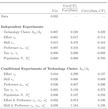
ratioV ar(CF)/V ar(Data), 0.228, indicates that its impact is not negligible.
The importance of technology choice in understanding the cross-country variation in the time
technology choice. However, a negative correlation,−0.164, suggests that skill itself cannot explain the observed cross-country variation. Among the other sources affecting the time gap through general equilibrium effects only, preference has comparable numbers for both the variance ratio and
correlation, 0.216 and 0.242, respectively. Effort, tax and population, the first of which is closely related to the couple households, have negligible impacts on the time gap because the variance ratio
is relatively small compared with that of technology choice.
This conclusion is robust in the sense that neither the correlation Corr(Data, CF) nor vari-ance ratio V ar(CF)/V ar(Data) change significantly, even if we allow for additional variations in the other sources of the gender gaps. As demonstrated in Table 2 (which reports the results of several conditional experiments), the correlation Corr(Data, CF) between the data and counter-factual remains positive and range from 0.089 for the skill gap to 0.372 for tax, and the variance ratio V ar(CF)/V ar(Data) is also far from zero, ranging from 0.158 for tax to 1.184 for skill and preference.
3.5 Couple Time Gap
We also assume a southeast shift of technology (Am/Af) on the U.S.-equivalent frontier. Then, unlike the single household, we should observe a clear-cut relationship between the associated in-crease in the efficiency wage gapwm/wf and the time gaphN,m/hN,f. According to (13), the couple household chooses its members’ time devoted to home production such that the female engages in home production more than the male, or stated differently, the time gap hN,m/hN,f is negatively correlated with the efficiency wage gap wm/wf. Intuitively, market goods, g, are shared as public goods within the households through cooperation between members and the effects of
complemen-tarity between market goods and time devoted to home production on the time gap thus cancel out across members; thus, only the effects of the opportunity costs prevail and result in a perfect log-linear relationship between the time and wage gaps.
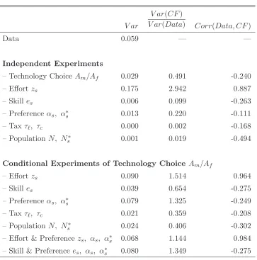
To what extent can this cross-country variation in the time gap induced by technology choice explain the actual variation? Notably, the results contrast with the case of the single household.
The independent experiment indicates that the correlation Corr(Data, CF) between the data and counterfactual is negative, with a value of approximately −0.240, as shown in Table 3 or observed in the right panel of Figure 2, which suggests that technology choice cannot explain the observed
cross-country variation in the time gap by itself. Thus, the observed cross-country variation in the time gap of the couple household is driven by some factor(s) whose effects are negatively correlated
with the effects of technology choice.
However, this result does not indicate that technology choice is not an important source of the
household. Table 3 reports that the variance ratio is approximately 0.491. This effect is robust in
the sense that the variance ratio does not change significantly and instead increases when combined with other sources of the cross-country variation of the gender gaps, as observed in conditional
experiments.
In addition, technology choice is also important in the sense that there is no single factor that can
explain the actual cross-country variation in the time gap of the couple households. Although effort
zs has a correlation Corr(Data, CF) between the data and counterfactual that is sufficiently close to one, its variance ratio V ar(CF)/V ar(Data) is too large to explain the cross-country variation. Instead, the combination of technology choice and effort or the triplet of technology choice, effort and preference has a variance ratio and correlation closer to one compared with those of either
technology choice or effort by itself, which implies that without technology choice it is difficult to explain the cross-country variation in the time gap without technology choice. Among these
parameters, the latter explains the cross-country variation the most with a variance ratio of 1.144 and correlation of 0.984.
The above results thus suggest that the mechanisms that determine the time devoted to home
production are crucially different across different types of households not only in the sense that the cooperation between members makes the net effects of the opportunity costs larger but also in the
sense that the actual cross-country variation in the time gap of the couple household deviates from the prediction with technology choice only to a small extent. An immediate implication of this result is that the global policy trend, which is expected to narrow gender gaps by affecting technology
choice and is characterized by the convergence in Am/Af, might not achieve smaller wage and time gaps simultaneously (at least for couple households). As demonstrated by the independent and
conditional experiments, the cross-country variation in technology choiceAm/Af offsets the cross-country variation in the time gap of the couple households which is widened by the cross-cross-country
variation in effortzs. Thus, if theAm/Af values of countries converge, the effect of effort becomes larger, resulting in a wider cross-country variation in the time gap. This result indicates that in some countries, the time gap will become narrower, whereas other countries will experience larger
time gaps.16
4
Robustness Analysis
We performed sensitivity checks by changing parameter values, assumptions and utility function
specifications within the context of the baseline. Tables 4–6 compare the results when the main
16 As demonstrated in Section 4, the result that the correlation between couple time gaps from the data and
counterfactual under the inappropriate technology choice is negative and robust to different parameter values and specifications. Thus, stated differently, the implication that a convergence in Am/Af results in a divergence in the
Wage Gap, wmem/(wfef) Time Gap (Single),h∗N,m/h∗N,f Time Gap (Couple),hN,m/hN,f 0.5 1 1.5 2 m f 0.2 0.4 0.6 0.8 1 m f 0 0.5 1 1.5 m f A U S D E U I T A J P N N L D E P S G B R U S A A U S D E U I T A J P N N L D E P S G B R U S A A U S D E U I T A J P N N L D E P S G B R U S A Data CF
Figure 2: Effects of Technology Choice on the Gender Gaps: Independent Experiment
Notes: Figure shows the male-female to ratio for each variable. The green open circles are the counterfactual simulation
results that are represented.
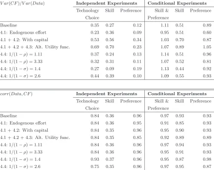
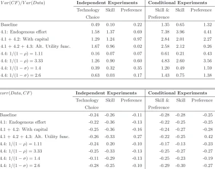
experiments are implemented under alternative assumptions. These results indicate that firm tech-nology choice can explain the cross-country variance to some extent, even under different
assump-tions; thus, we concluded that firm technology choice has a significant impact on the gender wage and time gaps.
Specifically, we conduct four types of sensitivity experiments:
1. Endogenous Home Production Effort
2. With Physical Capital Model
3. Composite Type Utility Function
4. Changing Elasticity of Substitution Values
Different from calibration forms and simulation algorithms of the baseline model are discussed in Appendix D.
4.1 Endogenous Home Production Effort
Thehome production effort, or simplyeffort,zsis given exogenously in the main experiments: thus, even, when a firm changes its technology choice, the home production effort does not change. For example, if a firm decides to enhance life-work balance to help female workers, the couple household may change each spouse’s function and the husband may work more in home production, in which
case, the male’s home production effort will increase due to the changing comparative advantage. In this subsection, we examine such an effect for effort. The couple household can select the effort
[image:19.612.84.516.70.237.2]technology choice problem. The couple household maximizes its utility function subject to the
following constraint
zωH
m +υHzfωH ≤BH (18)
and those that appear in the benchmark case. This constraint plays a similar role as in technology choice problem of the firm side. BH is the inverse measure of the barrier to a household technology frontier,υH is the relative cost of shifting to spouse’s home production productivity andωH governs the curvature of the household technology frontier. If ρ >0, which is the case that we consider in this paper, then ωH >1 guarantees an interior solution of the household.
Considering the FOCs with respect tozm and zf and taking the ratio of this equation for each sex s,
zm
zf =υ
1−ρ
(1−ρ)ωH−1
H
µ
wm
wf
¶−(1−ρ)ρ
ωH−1
,
implies that the home production effort changes due to the comparative advantage of market work.
When we calibrate zm and zf using the data, we restrict ourselves to zm+zf = 1 as the main experiment settings to identify these parameters. However, when performing simulations, we can identify these parameters without this restriction, i.e.,zm+zf 6= 1.
4.2 With Physical Capital Model
In this subsection, the endogenous home production effort model is further extended to include
capital stock that is given exogenously. Each household has one unit of capital stockkand rents it to firms at rental rater.17 The total capital stock NkequalsK. The couple and single households’
budget constraint are added capital income,
Couple household: (1 +τc)g≤(1−τℓ)(wmemhM m+wfefhM f) + (1−τk)2rk+ 2T, (19) Single household: (1 +τc)gs∗ ≤(1−τℓ)wsesh∗M,s+ (1−τk)rk+T, (20)
where τk is the capital income tax, r is the rental rate of capital and k is the per capita physical capital,k≡K/N.
The government’s budget constraint also changes when including capital income tax revenue,
NT =N τcg+ X
s∈{m,f}
Ns∗τcg∗s+
X
s∈{m,f}
N τℓwseshM,s+
X
s∈{m,f}
Ns∗τℓwsesh∗M,s+τkK. (21)
The FOCs of the household are the same as in the main model.
17 We assume that each type of household has the same amount of capital stock, because we cannot observe a
Firms then use capital, labor, and technology to produce output according to the two-tier
production function,
max
K, {Ls, As, K}s∈{m,f}
{Y −wmLm−wfLf −rK},
Y =Kθ[(AmLm)σ+ (AfLf)σ]
1−θ
σ (22)
s.t. Aωm+υAωf ≤B,
where θis the capital share and 0< θ <1.
The equilibrium definition is discussed in Appendix D.2.
4.3 Composite-type Utility Function
The utility function in the baseline model is separable between consumption and leisure and also
between spouses. We examine whether we would obtain the same results under different specifica-tions for the household utility function. In this subsection, we selected the following specification, which addresses the composite hours of leisure between husband and wife:
max
X
s∈{m,f}
αsln(cs) +bln
n
[am(1−hM,m−hN,m)ǫ+af(1−hM,f −hN,f)ǫ]
1
ǫ
o
, (23)
where ǫ <1 governs the elasticity 1/(1−ǫ) between the male and female in leisure activities.
4.4 Elasticity of Substitution
Unfortunately, to our knowledge, there are no empirical studies on the elasticity of substitution of home production between couples, i.e., 1/(1−ρ). However, previous studies of the gender gap provide this elasticity with a lack of foundation. However, the sharing roles of home production might be affected by this elasticity. Therefore, we verified the sensitivity of the value of elasticity.
In addition, a few empirical works have estimated the elasticity of substitution between male
labor and female labor, 1/(1−σ). Our baseline simulation is based on the mean value of these studies, and we verified the sensitivity of this value.
4.5 Results
We conduct several alternative specification and parameters checks to verify the robustness of the
findings reported above. We do not experiment with effort because home production effort is determined endogenously in these models, with the exception of the baseline model. Tables 4–6
5
Conclusion
To what extent and how does firm technology choice affect the cross-country variations in the gender
gap in wage and time allocation?
To answer this question, we build a general equilibrium model of the gender wage gap and time allocation with technology choice and home production of households with different marital
statuses. Firms choose their production technology depending on the relative abundance of labor for each sex and the relative costs of shifting their technology.
The main finding is that technology choice has considerable impacts on the cross-country vari-ation in not only the gender wage gap but also the gender difference of time allocvari-ation, which implies that the effects of a policy aiming to narrow the gender gaps are gradual because the policy
must face firms’ technology choice, including the labor market institutions, corporate culture, and social norms, which are difficult to change dramatically. Our findings also indicate that there is no
single mechanism determining the observed cross-country variations in gender gaps. Therefore, a convergence in the technology choice across countries itself does not result in a convergence in all
the gender gap measures in general, which suggests that policy makers should set multiple targets when intending to narrow all gender gap measures.
A possible extension of this study would be to introduce bargaining into the household problem
by considering the literature of the collective model (cf. Bourguignon et al. (2009)).
References
Acemoglu, Daron (2002) “Directed Technical Change,” Review of Economic Studies, Vol. 69, No.
4, pp. 781–809, October.
Acemoglu, Daron, David H. Autor, and David Lyle (2004) “Women, War, and Wages: The Effect
of Female Labor Supply on the Wage Structure at Midcentury,” Journal of Political Economy, Vol. 112, No. 3, pp. 497–551, June.
Aguiar, Mark and Erik Hurst (2007) “Life-Cycle Prices and Production,” American Economic
Review, Vol. 97, No. 5, pp. 1533–1559, December.
Arrow, Kenneth (1971) “The Theory of Discrimination,” Working Papers 403, Princeton University,
Department of Economics, Industrial Relations Section.
Becker, Gary S. (1965) “A Theory of the Allocation of Time,”Economic Journal, Vol. 75, No. 299, pp. 493–517, September.
Blau, Francine D. and Lawrence M. Kahn (1992) “The Gender Earnings Gap: Learning from
International Comparisons,”American Economic Review, Vol. 82, No. 2, pp. 533–538, May.
(1995) “The Gender Earnings Gap: Some International Evidence,” in Richard B. Freeman and Lawrence F. Katz eds.Differences and Changes in Wage Structures, Chicago: University of
Chicago Press, Chap. 3, pp. 105–144.
(1996a) “International Differences in Male Wage Inequality: Institutions versus Market
Forces,”Journal of Political Economy, Vol. 104, No. 4, pp. 791–836, August.
(1996b) “Wage Structure and Gender Earnings Differentials: An International Compari-son,” Economica, Vol. 63, No. 250, pp. S29–62, Suppl.
(1999) “Institutions and laws in the labor market,” in O. Ashenfelter and D. Card eds. Handbook of Labor Economics, Vol. 3: Elsevier, Chap. 25, pp. 1399–1461.
(2003) “Understanding International Differences in the Gender Pay Gap,”Journal of Labor
Economics, Vol. 21, No. 1, pp. 106–144, January.
Boeri, Tito (2011) “Institutional Reforms and Dualism in European Labor Markets,” in O. Ashen-felter and D. Card eds.Handbook of Labor Economics, Vol. 4: Elsevier, Chap. 13, pp. 1173–1236.
Bourguignon, Franc¸ois, Martin Browning, and Pierre-Andr´e Chiappori (2009) “Efficient Intra-Household Allocations and Distribution Factors: Implications and Identification,” Review of
Economic Studies, Vol. 76, No. 2, pp. 503–528, April.
Caselli, Francesco and Wilbur John Coleman (2006) “The World Technology Frontier,” American Economic Review, Vol. 96, No. 3, pp. 499–522, June.
Chang, Yongsung and Frank Schorfheide (2003) “Labor-supply shifts and economic fluctuations,” Journal of Monetary Economics, Vol. 50, No. 8, pp. 1751–1768, November.
Flabbi, Luca (2010) “Prejudice and gender differentials in the US labor market in the last twenty
years,”Journal of Econometrics, Vol. 156, No. 1, pp. 190–200, May.
Gronau, Reuben (1977) “Leisure, Home Production, and Work-The Theory of the Allocation of Time Revisited,”Journal of Political Economy, Vol. 85, No. 6, pp. 1099–1123, December.
(1980) “Home Production-A Forgotten Industry,”The Review of Economics and Statistics, Vol. 62, No. 3, pp. 408–416, August.
Gronau, Reuben and Daniel S. Hamermesh (2008) “The Demand for Variety: A Household
Gupta, Nabanita Datta and Donna S. Rothstein (2005) “The Impact of Worker and
Establishment-level Characteristics on Male-Female Wage Differentials: Evidence from Danish Matched Employee-Employer Data,”LABOUR, Vol. 19, No. 1, pp. 1–34, March.
Jones, Charles I. and Paul M. Romer (2010) “The New Kaldor Facts: Ideas, Institutions, Population,
and Human Capital,”American Economic Journal: Macroeconomics, Vol. 2, No. 1, pp. 224–45, January.
Jones, Larry E., Rodolfo E. Manuelli, and Ellen R. McGrattan (2003) “Why are married women
working so much?” Staff Report 317, Federal Reserve Bank of Minneapolis.
Layard, Richard (1982) “Youth Unemployment in Britain and the United States Compared,” in Richard B. Freeman and David A. Wise eds. The Youth Labor Market Problem: Its Nature,
Causes, and Consequences, Chicago: University of Chicago Press, Chap. 15, pp. 499–542.
Lazear, Edward P and Sherwin Rosen (1990) “Male-Female Wage Differentials in Job Ladders,” Journal of Labor Economics, Vol. 8, No. 1, pp. 106–123, January.
Lewis, Philip E. T. (1985) “Substitution between Young and Adult Workers in Australia,”Australian Economic Papers, Vol. 24, No. 44, pp. 115–126, June.
McDaniel, Cara (2007) “Average tax rates on consumption, investment, labor and capital
in the OECD 1950-2003,” March. Arizona State University, paper and data available at http://www.caramcdaniel.com/researchpapers.
(2011) “Forces Shaping Hours Worked in the OECD, 1960-2004,” American Economic
Journal: Macroeconomics, Vol. 3, No. 4, pp. 27–52, October.
McGrattan, Ellen R., Richard Rogerson, and Randall Wright (1997) “An Equilibrium Model of the Business Cycle with Household Production and Fiscal Policy,”International Economic Review, Vol. 38, No. 2, pp. 267–290, May.
Meyersson-Milgrom, Eva M., Trond Petersen, and Vemund Snartland (2001) “Equal Pay for Equal Work? Evidence from Sweden and a Comparison with Norway and the U.S,” Scandinavian Journal of Economics, Vol. 103, No. 4, pp. 559–83, December.
Nickell, Stephen and Richard Layard (1999) “Labor market institutions and economic performance,” in O. Ashenfelter and D. Card eds.Handbook of Labor Economics, Vol. 3 of Handbook of Labor Economics: Elsevier, Chap. 46, pp. 3029–3084.
Olivetti, Claudia and Barbara Petrongolo (2008) “Unequal Pay or Unequal Employment? A
Cross-Country Analysis of Gender Gaps,” Journal of Labor Economics, Vol. 26, No. 4, pp. 621–654, October.
(2011) “Gender Gaps across Countries and Skills: Supply, Demand and the Industry
Struc-ture,” NBER Working Papers 17349, National Bureau of Economic Research, Inc.
Olovsson, Conny (2004) “Why do Europeans Work so Little?” Seminar Papers 727, Stockholm
University, Institute for International Economic Studies.
O’Neill, June (2003) “The Gender Gap in Wages, circa 2000,”American Economic Review, Vol. 93, No. 2, pp. 309–314, May.
Pfeifer, Christian and Tatjana Sohr (2009) “Analysing the Gender Wage Gap (GWG) Using Per-sonnel Records,”LABOUR, Vol. 23, No. 2, pp. 257–282, June.
Prescott, Edward C. (2004) “Why do Americans work so much more than Europeans?” Quarterly
Review, No. 1, pp. 2–13, July.
Ragan, Kelly S. (2013) “Taxes and Time Use: Fiscal Policy in a Household Production Model,” American Economic Journal: Macroeconomics, Vol. 5, No. 1, pp. 168–92, January.
Rogerson, Richard (2009) “Market Work, Home Work, and Taxes: A Cross-Country Analysis,” Review of International Economics, Vol. 17, No. 3, pp. 588–601, August.
Rupert, Peter, Richard Rogerson, and Randall Wright (1995) “Estimating Substitution Elasticities
in Household Production Models,”Economic Theory, Vol. 6, No. 1, pp. 179–193, January.
Weinberg, Bruce A. (2000) “Computer use and the demand for female workers,” Industrial and Labor Relations Review, Vol. 53, No. 2, pp. 290–308, January.
Appendix A
Data
Appendix A provides details of the data that we used for calibration and simulation.
Appendix A.1 Gross Domestic Product
Appendix A.2 Time Allocation
The data source of time allocation differs depending on the country. We used the Survey on
Time Use and Leisure Activities for Japan and the Multinational Time Use Study(MTUS) for all other countries. The procedure for the construction of time allocation consistent with the model is
discussed below for each statistic.
Appendix A.2.1 Multinational Time Use Study (MTUS)
The time allocation data for market working hours and home production hours were obtained from the MTUS. This dataset contains the time allocation of individuals among countries. There are
several versions of the data available, such as World 5.53, World 5.8, and World 6.0. The differences among these three versions include that the latter two versions include participants under 18 and the
time allocation data are presented in a more detailed manner, whereas the data in World 5.53 are categorized more broadly. By dividing the time allocation of a day into three blocks, namely, market
work, home production, and leisure, World 5.53 fully satisfies our aim. The countries included in World 5.53 are listed in Table 7.
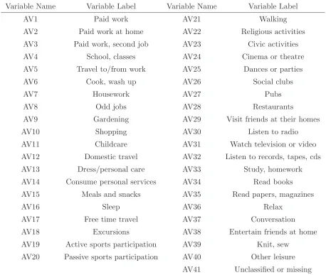
MTUS time use data are provided in the form of a diary collected from individuals. The records of one’s behaviors are divided into 41 harmonized activities, and the amount of time allocated
(measured in minutes) for each activity is available. Therefore, we constructed the definition of time allocation for market work, home production, and leisure and reallocated the former 41 activities into each category. Specifically, we selected four variables to indicate market work, five variables to
indicate home production, and the remaining variables to indicate leisure. Details are provided in Tables 8 and 9.
Next, we describe the methodology for constructing the time use data consistently for our analysis. We excluded individuals who were not employed (including retired people) and only used
individuals in the range of 20 to 60 years old. Both students and individuals with military duty were omitted. In addition, we ignored the diaries recorded on weekends, as well as people working less than 25 hours per week or working more than 70 hours per week. The upper bound for home
production hours was set to 10 hours per day. After filtering out the noisy samples, we were left with countries that had a sufficient sample size for constructing our time allocation data.
The method of construction the time allocation variables is fairly simple. We aggregate all the individuals’ time allocations from their diaries that satisfied our requirements and employed the
Appendix A.2.2 Survey on Time Use and Leisure Activities
We obtained the time allocation data for Japan from the aggregated data of the Survey on Time
Use and Leisure Activities (Ministry of Internal Affairs and Communications, Statistics Bureau of Japan.). The construction methods for our variables are almost the same as MTUS. We defined
worked hours as the market working hours hM,s {s ∈ m, f}, and housework as home production hours hN,s {s∈m, f}. The data are presented in Table 12.
Appendix B
Calibration
In this section, we describe the detailed procedure of our calibration. Table 13 presents all the
variables in the baseline model. Variables are classified into three types: “Data” represents the variables given by data directly, “Exogenous parameters” are mainly taken from previous studies,
and “Calibrated parameters” are determined from the equations presented below.
We first calibrate the household structure ({Ns∗}s∈{m,f}, N) and skill{es}s∈{m,f}, and tax rates
(τc, τL), which are independently calibrated. Then, given the result and also the fixed exogenous parameters, we calibrate the firm-side parameters. Finally, we calibrate the remainder of the pa-rameters on the household side.
Appendix B.1 Independently Calibrated Parameters Household Structure
The main purpose of our paper is to investigate the aggregate gender gap, which requires the
male-female ratio of the labor supply in our model to match the data. To achieve this requirement, we calibrate the household structure to fit the male-female ratio of the labor supply data. Our model’s
population consists of three groups: couple households N with a male and a female, male single households Nm∗ and female single households Nf∗, the members of which consist of only a male or only a female, respectively; thus, we calibrate the three parameters N, Nm∗, Nf∗. Regarding the matched labor supply ratio, we also uses the Census of each country to calibrate the data to fit the Census household structure as much as possible. We use the household structure as target in
addition to the labor supply ratio because the household structure system in our model requires two calibration targets to satisfy the rank conditions.
Except for Japan and the U.S., we use EU statistics on income and living conditions, which reports the distribution of population by household type. This database contains no information about the age profile and presence or absence of children by gender for a single person. Therefore,
we assume that a single person with dependent children has the same ratio by gender. We calculated
× Single person by sex ratio, N = Two adults younger than 65 years.
Japan’s household structure data are obtained from the Ministry of Internal Affairs and
Com-munications, Census, 2005 and the U.S. data are obtained from the Census Bureau, Statistical Abstract of the United States, 2009. We use the following figures:
Ns∗ = Household living alone by sex, N = Married Couple without children.
Finally, we normalize the total number of householdsN=P
s∈{m,f}Ns∗+N to unity.
Skill
Skilles is calibrated by human capital accumulated in schooling. Specifically, we employ a method-ology similar to that reported in Caselli and Coleman (2006) to construct the skill data using EU
KLEMS (Release March 2008). As discussed above, skill is defined as a weighted sum of the daily working hour ratio per worker, in which the workers are divided into three groups based on their
re-spective schooling: low, medium and high education. We set the low educated group as the baseline and take a weighted sum of the medium- and high-educated workers relative to the low-educated workers. The weight for the accumulation of a group is its relative labor income per unit of working
hours to the baseline group. The skill measure is independently constructed for males and females, and each skill is normalized by the total sum of both efficiency units.
Tax Rates
Both consumption and labor income tax rates are acquired from McDaniel (2007), who provides these tax rates as well as the taxes on investment and capital for 15 OECD countries.
Appendix B.2 Firm-side Parameters
For the firm-side parameters, we first calibrate the hourly gender wage gap wmem/(wfef), and fix the value of the elasticity of substitution between the market hours of males and females, 1/(1−σ). Then, using these results as well as those of the independently calibrated parameters and MTUS, we calibrate (Am, Af) for eight countries. Finally, we conduct a regression to obtain the values of (ω, υ, B) under a certain assumption.
Hourly Gender Wage Gap