Munich Personal RePEc Archive
An experimental investigation of
auctions and bargaining in procurement
Shachat, Jason and Tan, Lijia
Wang Yanan Institute for Studies in Economics, Xiamen University
17 October 2012
An experimental investigation of auctions and
bargaining in procurement
Jason Shachat
∗Lijia Tan
†October 17, 2012
Abstract
In reverse auctions, buyers often retain the right to bargain further concessions from the winner. The optimal form of such procurement is an English auction followed by an auctioneer’s option to engage in ultimatum bargaining with the winner. We study behavior and performance in this procurement format using a laboratory experiment. Sellers closely follow the equilibrium strategy of exiting the auction at their costs and then accepting strictly profitable offers. Buyers generally exercise their option to bargain according to their equilibrium strategy, but their take-it-or-leave-it offers vary positively with auction prices when they should be invariant. We explain this deviation by modeling buyers’ subjective posteriors regarding the winners’ costs as distortions, calculated using a formulation of probability weighting, of the Bayesian posteriors. We show alternative models based upon risk aversion and anticipated regret can’t explain these price dependencies.
JEL classifications: C34; C92; D03; D44
Keywords: Auction, Bargain, Experiment, Subjective Posterior
∗The Wang Yanan Institute for Studies in Economics, and MOE Key Laboratory in Econometrics, Xiamen
University,[email protected]
1
Introduction
Auctions that set a benchmark price and award exclusive rights to negotiate a final purchase contract are commonly used in many areas of commerce such as procurement in supply chains (Tunca and Wu, 2009; Elmaghraby, 2007), corporate mergers and acquisitions (Hege, Slovin, B., and Sushka, 2009), and even professional sports teams exchanging the rights of players.1
A seminal article by Bulow and Klemperer (1996) shows that conducting a reverse (forward) English auction with the auctioneer retaining the right to make a take-it-or-leave-it offer to the auction winner implements the optimal mechanism - Myerson (1981) - to sell (purchase) an object. Furthermore, they establish the auctioneer’s expected welfare increases by fore-going this auction-bargaining mechanism and instead conducting an English auction with an additional serious bidder. Unfortunately, identifying and validating additional serious bidders is often cost prohibitive and difficult, particularly in the procurement setting (Wan and Beil, 2009; Wan, Beil, and Katok, Forthcoming). Consequently, evaluating behavior and performance in Bulow and Klemperer’s auction-bargaining mechanism within a procurement setting is an important task.
The Nash equilibrium, implementing the optimal mechanism outcome, has a simple struc-ture but also relies upon some behaviorally questionable assumptions. A seller’s strategy is to exit the auction when her costs exceeds the auction price, and accept any subsequent profitable ultimatum offer. This opposes what is observed in ultimatum game experiments where responders commonly reject profitable offers that are less than equitable even when experienced (Cooper and Dutcher, 2011), or there is incomplete information about amount of potential social surplus (Croson, 1996; Harstad and Nagel, 2004).2 In our experiment, seller’s
generally exit the auction at their cost, and they rarely reject profitable take-it-or-leave-it offers.
The buyer’s equilibrium strategy is characterized by a price threshold that is conditional upon his willingness-to-pay. He accepts an auction outcome when the price is below his threshold; otherwise, he makes a take-it-or-leave-it offers equal to the threshold. Both the auction-bargaining mechanism and the more commonly considered English auction with an optimal reserve price implement the optimal direct mechanism. Therefore the buyer’s threshold price in the auction-bargaining mechanism is exactly the optimal reserve price in
1For example the Nippon Professional Baseball League and Korean Baseball Organization have a posting
system, that allows a player to ask his current team to conduct an auction granting a period of exclusive negotiating rights to a Major League Baseball team; about one player per year leaves the Nippon League through this process. An even more relevant practice - in which no compensation occurs in absence of a final contract - is trade of players between teams in the National Basketball Association or National Football League conditional upon the player and new team agreeing to a contract extension.
the English auction. This implies the threshold price is independent of the realized auction price, and depends only upon the buyer’s value and the distribution of the sellers’ costs. This seems almost paradoxical as, unlike an reserve price, the buyer only commits to a threshold after the auction, thus gaining additional information about the winning seller’s cost. We show the invariance of the price threshold to the realized auction price relies upon the buyer forming correct Bayesian posterior beliefs regarding the lowest cost conditional the realized second lowest cost, i.e. the auction price.
While the buyer’s strategy accurately predicts rejected auction outcomes subsequent take-it-or-leave-it offers have a strong positive relationship with the auction price - contra-dicting the prediction of price invariance. This results in reducing consumer surplus by approximately 7.5%. Further there is substantial individual heterogeneity in this sensitivity to auction price.
We find an explanation for this behavior by generalizing how a buyer formulates his posterior belief regarding the auction winner’s cost conditional upon the auction price. We propose the subjective posterior is formed by applying the two-parameter Prelec (1998) prob-ability weighting function to transform the Bayesian posterior. This allows the subjective posterior to flexibly reflect differing types of perceived affiliation between the auction price and winner’s cost. Structural estimates of this model demonstrate its ability to capture both the observed wide varying pattern of buyer behavior and the general property of the positive relationship between auction price and bargaining offers. We further show that sim-ply allowing for risk aversion does not lead to any relationship between auction price and bargaining offers, and anticipated regret only leads to a negative relationship. Thus, of these three alternatives, our subjective posterior model is the only plausible explanation.
2
Basic theory
We present an alternative demonstration of the equilibrium for the auction-bargaining format that elucidates the role of how the buyer dynamically processes information.3 Through this
presentation we can highlight how different behavioral biases impact the optimality of the buyer’s decisions.
Consider a buyer who desires an indivisible object. His value for this object is the random variable v with the absolutely continuous distribution function H(v) on the interval [v, v],
v > 0, and associated probability distribution function h(v). Only the buyer knows his
3Note that both Bulow and Klemperer (1996) and Myerson (1981) consider the strategically equivalent
realized valuation. There areN possible sellers, indexed by i. Upon selling an object, seller
i incurs a unit cost ofci. Each seller’s unit cost is an independent random variable with the common absolutely continuous distribution function F(c) on the interval [0, c], with c < v, and associated probability distribution functionf(c). We also assumes thatc+Ff((cc)) is strictly increasing on the support of F. Only a seller knows her realized cost, which she learns prior to any strategic interaction. H(v) and F(c) are also independent, so a seller’s realized cost reveals no additional information about the buyer’s value.
Here are the specific rules of the auction-bargaining mechanism. First, the sellers compete in a reverse English clock auction in which price starts atc and all N sellers in the auction. Price falls with time, and a seller can irreversibly exit the auction at any time. The auctions closes, and the auction price p determined, when either N −1 sellers have exited or price reaches zero. Ties in either being the N −1 seller to exit, or multiple winners at a price of zero are settled randomly. Any seller who does not win the auction receives a payoff of zero. The buyer is informed of the auction price and chooses to either accept the auction price, resulting in payoffs of v−p for the buyer and p−ci for the winner, or makes a take-it-or-leave-it offer o to the winner. In the case of the latter, the winning seller either accepts the offer, resulting in payoffs ofv−o and o−ci, or rejects the offer and all parties receive a zero payoff.
A seller’s strategy has two parts: a function that maps from possible unit costs to auction exit prices; and a function that maps from possible counter-offer information sets to reject and accept decisions. The buyer’s strategy is a function that maps from possible value and auction price pairs to possible counter offers join with accepting the auction outcome. We now show the strategy profile in which each seller exits the auction at her unit cost and then accepts any profitable take-it-or-leave-it offer, and the buyer accepts all auction prices below some threshold level - conditional onv - otherwise making an optimal counter offer is a Nash equilibrium.
Consider the optimality of the buyer’s strategy conditional upon those of the sellers. The buyer’s conditional payoff function is
π(o|v, p) = max{v−p,max(v−o)G(o|p)}. (1)
G(o|p) is the buyer’s subjective probability distribution of the auction winner’s cost which need be not derived according to Baye’s rule, but o+Gg((oo||pp)) must be strictly increasing. The first order condition for an interior maximum of the second argument of (1) implies,
v−o∗ = G(o
∗|p)
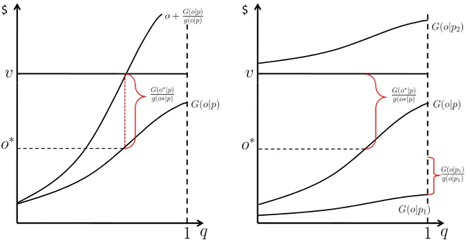
We provide an economic interpretation of Equation (2) from the theory of a price setting monopsonist; a direct analog to the classic interpretations of optimal forward auctions to monopoly theory (Bulow and Roberts, 1989; Bulow and Klemperer, 1996). If we define quantity as the probability the buyer procures the object, q = G(o|p), then the inverse average expenditure (market supply) function isG(o|p), and the inverse marginal expenditure function - expressed in terms of the monopsonist’s priceo- isM E(o) =o+Gg((oo||pp)). The buyer has a constant marginal value of v for quantities between zero and one, implying a perfectly elastic demand curve at v in the same range. Now we can see the optimal markdown given in Equation (2), results from simply equating marginal value to marginal expenditure.
v =o∗+G(o∗|p)
g(o∗|p).
The relationship between v, average expenditure, and marginal expenditure are depicted in the left hand graph of Figure 1. There are also two types of corner solutions: the buyer’s believes with probability zero that the winner’s cost is below his value and thus o∗ = v,
and when marginal expenditure never exceeds v in which case o∗ = G−1(1|p). All three
types of solutions are depicted in the right hand graph of Figure 1. When determining whether to accept the auction outcome or engage in bargaining, he simply compares whether
v−p≥(v−o∗)G(o∗|p).
If the auction-bargaining mechanism implements Myerson’s optimal mechanism, then the optimal counter offer implied in Equation (2) should be invariant to auction price. We can see this property is recovered whenever the buyer’s posterior regarding the auction winner’s cost satisfies the following property of conditional order statistics.
Proposition 1. Let ci, i = 1, . . . N, be independent realizations from the distribution F,
with ordering c1 ≤c2 ≤ · · · ≤cN, then the conditional distribution of c1 given c2, is the same
distribution as F truncated at c2.
Proof: This is Theorem 2.7 of David (1981).
If the buyer calculates his posterior according to Proposition 1 then,
v−o∗ = G(o
∗|p)
g(o∗|p) =
F(o∗)
F(p)
f(o∗)
F(p)
= F(o
∗)
f(o∗). (3)
Note the corner solution where marginal expenditure does not exceed v occurs when p≤o∗
and G(o∗|p) = 1. In this case it is clear that v−p≥ v −o∗, and the buyer maximizes his
Figure 1: Optimal offer: the left graph illustrates an interior solution. The right graph illustrates an interior solution at auction price p, a corner solution at p1 where marginal
expenditure never crosses v and o∗ = G−1(1|p
1), and another corner solution for p2 where
G−1(0|p
2)> v and o∗ =v.
$ $
The seller’s strategy is an optimal response given the buyer’s strategy because she can never strictly increase her payoff by accepting an offer above her cost, nor by rejecting one above her cost. Correspondingly, exiting the auction at her cost is optimal by standard arguments (for example, see Krishna (2009) page:15) for the exiting at cost in typical private cost English auctions.
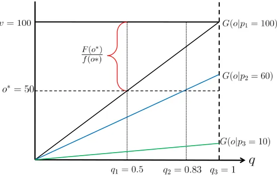
Consider the following example which is also the setting we use in our experiment. The distribution of the buyer’s value H(v) is the uniform distribution on [50,150]. There are two sellers and F(c) is the uniform distribution on [0,100]. For a realized value v, by Equation (3), o∗ = v/2. So while the optimal threshold does not depend upon price, the
Figure 2: The optimal offer for v = 100 and F(c) = c
100. For p > 50 the optimal counter
offer is 50 and does not vary with the price, but the corresponding probability of purchasing,
G(50|p) does. For p≤50 the buyer accepts the auction outcome.
$
3
Experimental design and hypotheses
3.1
Experimental design
Our experiment consists of the following session flow. First, we recruit 18 subjects to par-ticipate in a two hour experimental session. We randomly designate 6 subjects as buyers and 12 subjects as sellers; these designations are fixed for the session. The session consists of 2 practice periods and 30 rounds for which subjects receive compensation based upon their decisions. Every period we randomly form 6 trios consisting of 2 sellers and 1 buyer. Participants are informed of the random rematching protocol and that all costs and values are redrawn each period.
Each trio plays the previous example of auction-bargaining mechanism, and we induce common knowledge by publicly reading and displaying instructions at the start of the ex-periment.4 The periods starts with each buyer and seller learning their respective value
and cost for this period. The two sellers in a trio participate in a descending English clock auction - without knowing the buyer’s realized value. The initial auction price is $100 and decrements by $ 1 every 0.7 second. When a seller exits the auction, the auction concludes with winner and price determination as previously indicated.5 Next, the buyer is informed
of his auction price and presented the choice to either accept the auction outcome or make a
4Instructions are available upon request from the authors.
take-it-or-leave-it offer to the auction winning seller. If he accepts the auction outcome, all trio members are informed of their payoffs and the period concludes. If the buyer instead engages in bargaining, the auction winner is presented with the counteroffer and decides whether to accept or reject. In either case, payoffs are reported and the period ends.
We conducted 8 sessions at the Finance and Economics Experimental Laboratory (FEEL) at Xiamen University.6 This gives us a total of 144 subjects (48 buyers and 96 sellers) each
with 30 observations. Subjects on average earned 70 RMB for their participation. We recruited subjects through the ORSEE system (Greiner, 2004), all of whom were undergrad-uate and gradundergrad-uate students enrolled in Xiamen University, and none had previous experience in this study. The experimental software was programmed in Z-tree (Fischbacher, 2007).
3.2
Hypotheses
Our ex ante hypothesis consists of one regarding economic performance and three regarding buyer and seller behavior. The main result of the Bulow and Klemperer (1996) study is that while the auction-bargaining mechanism increases the auctioneer’s expected payoff from a simpleN-bidder English auction, it fails to offer the auctioneer less value than adding another serious bidder7 and conducting a N + 1 bidder English auction.
Hypothesis 1. Buyer profit is greater than expected profit in a two-bidder English auction and less than a three-bidder English auction.
Next, the Seller’s Nash equilibrium strategy we identified provides two additional hy-pothesize. This first is about seller’s behavior in the English auction phase.
Hypothesis 2. Sellers exit the auction at their realized costs.
Our prior for confirming this hypothesis is strong due to previous experimental results on independent private value forward auctions (Coppinger, Smith, and Titus, 1980) and private cost reverse auctions (Shachat and Wei, 2012). However, there is uncertainty regarding how the bargaining phase plays out and how this change in feedback affects the saliency of the seller optimal action in the auction. For example, a seller may ”overstay” in the auction if she believes with probability one there will be a counteroffer and an opportunity to reject it. Our second hypothesis about sellers concerns behavior when a seller confronts a take-it-or-leave-it offer.
6This facility is designed for the purpose of conducting economic experiments and has privacy carrels, a
private payment and sign-in area, and a separate monitor room from which the experimenter conducts the experiment.
7In our design, sometimes a seller fails to satisfy the serious bidder criteriac
i ≤v. However, our design
Hypothesis 3. Sellers don’t reject profitable offers, and reject non-profitable ones.
This hypothesis derived from sequential rationality has a stronger alternative hypothe-sis than it would appear at first glance. The bargaining phase of the game is strategically equivalent to an ultimatum game in which the buyer and seller only respectively know the upper and lower ends of the ”pie” interval to be shared. The very large literature on Ul-timatum Game experiments, starting with Guth, Schmittberger, and Schwarze (1982), has shown that a non-negligible proportion of responders reject minimally profitable offers. In particular, this still holds true in studies that introduce asymmetric information about the pie size (Croson, 1996; Huck, 1999; Harstad and Nagel, 2004). However, a glaring coun-terexample are the results of Salmon and Wilson (2008) who study a two unit experimental English auction where the first unit is sold to the auction winner and a take-it-or-leave-it offer is made to last exiting bidder for the second unit. In this study, approximately only 4% of profitable offers where rejected. Our study is similar in that we imbed the ultimatum game as an after stage auction to determine possible responder participation. However, our setting differs as we have two-sided incomplete information and the responder does not have incentives to misrepresent her type (cost).
Our final hypothesis, developed in the previous section, regards the buyer’s behavior.
Hypothesis 4. Buyers follow their optimal strategy and implement the optimal auction.
4
Results
Our experimental data set consists of 1440 plays of the auction-bargaining mechanism, each including the losing seller’s exit price and the buyer’s decision of whether to bargain. Buyers chose to bargain 963 times, and the winning seller rejected the take-it-or-leave-it offer 280 of these times. We start buy comparing observed economic performance versus theoretical benchmarks for buyer profit, seller profit, and welfare improving trades. Then we examine the extent subjects follow their Nash equilibrium strategies.
4.1
Market performance
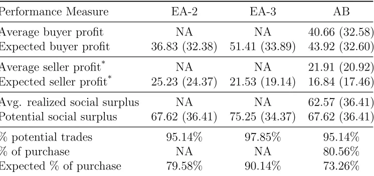
We start be presenting various summary statistics and their theoretical benchmarks in Ta-ble 1. When calculating the theoretical benchmarks for expected buyer and seller profit, and potential social surplus, max{0, v−min{ci}}, we use the realizations of the buyers’ values and sellers’ cost rather than the distributions they are drawn from.
Table 1: Realized Economic Performance (standard deviation)
Performance Measure EA-2 EA-3 AB
Average buyer profit NA NA 40.66 (32.58)
Expected buyer profit 36.83 (32.38) 51.41 (33.89) 43.92 (32.60)
Average seller profit* NA NA 21.91 (20.92)
Expected seller profit* 25.23 (24.37) 21.53 (19.14) 16.84 (17.46)
Avg. realized social surplus NA NA 62.57 (36.41)
Potential social surplus 67.62 (36.41) 75.25 (34.37) 67.62 (36.41)
% potential trades 95.14% 97.85% 95.14%
% of purchase NA NA 80.56%
Expected % of purchase 79.58% 90.14% 73.26%
* The auction winning seller.
EA-2 is English auction with two bidders, EA-3 is English auction with three bidders, AB is English auction with two bidders followed by take-it-or-leave-it bargaining.
Result 1. Using the auction-bargaining mechanism, buyer profit is greater than expected profit in a two-bidder English auction and less than a three-bidder English auction. Hypoth-esis 1 is confirmed by the t-tests of the third and fourth row of Table 2.
Table 2: P-values for t-tests between theoretical and observed profit
Role Null; Alternative t-statistic p-value
TAB = AAB; TAB 6= AAB −2.68 0.01
Buyer TEA-2 = AAB; TEA-2 <AAB −3.17 0.00
TEA-3 = AAB; TEA-3 >AAB 8.68 0.00
Auction TAB = AAB; TAB 6= AAB 7.05 0.00
Winning Seller TEA-2 = AAB; TEA-2 >AAB 3.92 0.00
TEA-3 = AAB; TEA-3 >AAB −0.51 0.70
TEA-2 is the expected profit in English auction with two bidders, TEA-3 is the expected profit in English auction with three bidders, AAB is observed average profit in English auction with two bidders followed by take-it-or-leave-it for bargaining for etake-it-or-leave-ither the buyer or auction winning seller.
[image:11.612.130.489.470.587.2]4.2
Seller behavior
Do sellers exit the auction when price reach their costs? Consider Figure 3, which plots the 1440 exit prices for the auction losing sellers versus their respective costs. There is a clear concentration of observations along the forty-five degree line. To provide quantitative evidence that sellers exit at price equals costs we conduct an ordinary least squares regression, finding an intercept of 3 and a slope coefficient of 0.95 (with an adjusted R2 statistic of 0.94). If we suppress the intercept term, then the slope coefficient is 0.99. These results are consistent with those previously found in English auctions in both forward (Coppinger, Smith, and Titus, 1980) and reverse (Shachat and Wei, 2012) contexts. Admittedly, there is some evidence that the potential bargaining phase leads to some overstaying in the auction for high costs, as seen in Figure 3, and noisy adherence to the equilibrium strategy. For example, the percentage of absolute deviations of bids from cost less than $1, $2, and $3 are respectively 56.5%, 75.0%, and 82.6%. With these minor caveats, we state our next result.
[image:12.612.159.441.391.653.2]Result 2. Sellers tend to exit the auction at their realized costs, confirming Hypothesis 2.
Figure 3: Auction exit price versus realized cost
● ● ● ● ● ● ● ● ● ● ● ● ● ● ● ● ● ● ● ● ● ● ● ● ●● ● ● ● ● ● ● ● ● ● ● ● ● ● ● ● ● ● ● ● ● ● ● ● ● ● ● ● ● ● ● ● ● ●● ● ● ● ● ● ● ● ● ● ● ● ● ● ● ● ● ● ● ● ● ● ● ● ● ● ● ● ● ● ● ● ● ● ● ● ● ● ● ● ● ● ● ● ● ● ● ● ● ● ● ● ● ● ● ● ● ● ● ● ● ● ● ● ● ● ● ● ● ● ● ● ● ● ● ● ● ● ● ● ● ● ● ● ● ● ● ● ● ● ● ● ● ● ● ● ● ● ● ● ● ● ● ● ● ● ● ● ● ● ● ● ● ● ● ● ● ● ●● ● ● ● ● ● ● ● ● ● ● ● ● ● ● ● ● ● ● ● ● ● ● ● ● ● ● ● ● ● ● ● ● ● ● ● ● ● ● ● ● ● ● ● ● ● ● ● ● ● ● ● ● ● ● ● ● ● ● ● ● ● ● ● ● ● ● ● ● ● ● ● ● ● ● ● ● ● ● ● ● ● ● ● ● ● ● ● ● ● ● ● ● ● ● ● ● ● ● ● ● ● ● ● ● ● ● ● ● ● ● ● ● ● ● ● ● ● ● ● ● ● ● ● ● ● ● ● ● ● ● ● ● ● ● ● ● ● ● ● ● ● ● ● ● ● ● ● ● ● ● ● ● ● ● ● ● ● ● ● ● ● ● ● ● ● ● ● ● ● ● ● ● ● ● ● ● ● ● ● ● ● ● ● ● ● ● ● ● ● ● ● ● ● ● ● ● ● ● ● ● ● ● ● ● ● ● ● ● ● ● ● ● ● ● ● ● ● ● ● ● ● ● ● ● ● ● ● ● ● ● ● ● ● ● ● ● ● ● ● ● ● ● ● ● ● ● ● ● ● ● ● ● ● ● ● ● ● ● ● ● ● ● ● ● ● ● ● ● ● ● ● ● ● ● ● ● ● ● ● ● ● ● ● ● ● ● ● ● ● ● ● ● ● ● ● ● ● ● ● ● ● ● ● ● ● ● ● ● ● ● ● ● ● ● ●● ● ● ● ● ● ● ● ● ● ● ● ● ● ● ● ● ● ● ● ● ● ● ● ● ● ● ● ● ● ● ● ● ●● ● ● ● ● ● ● ● ● ● ● ● ● ● ● ● ● ● ● ● ● ● ● ● ● ● ● ● ● ● ● ● ● ● ● ● ● ● ● ● ● ● ● ● ● ● ● ● ● ● ● ● ● ● ● ● ● ● ● ● ● ● ● ● ●● ● ● ● ● ● ● ● ● ● ● ● ● ● ● ● ● ● ● ● ● ● ● ● ● ● ● ● ●● ● ● ● ● ● ● ● ● ● ● ● ● ● ● ● ● ● ● ● ● ● ● ● ● ● ● ● ● ● ● ● ● ●● ● ● ● ● ● ● ● ● ● ● ● ● ● ● ● ● ● ● ● ● ● ● ● ● ● ● ● ● ● ● ● ● ● ● ● ● ● ● ● ● ● ● ● ●● ● ● ● ● ● ● ● ● ● ● ● ● ● ● ● ● ● ● ● ● ● ● ● ● ● ● ● ● ● ● ● ● ● ● ● ● ● ● ● ● ● ● ● ● ● ● ● ● ● ● ● ● ● ● ● ● ● ● ● ● ● ● ● ● ● ● ● ● ● ● ●● ● ● ● ● ● ● ● ● ● ● ● ● ● ● ● ● ● ● ● ● ● ● ● ● ● ● ● ● ● ● ● ● ● ● ● ● ● ● ● ● ● ● ● ● ● ● ● ● ● ● ● ● ● ● ● ● ● ● ● ● ● ● ● ● ● ● ● ● ● ● ● ● ● ● ● ● ● ● ● ● ● ● ● ● ● ● ● ● ● ● ● ● ● ● ● ● ● ● ● ● ● ● ● ● ● ● ● ● ● ● ● ● ● ● ● ● ● ● ● ● ● ● ● ● ● ● ● ● ● ● ● ● ● ● ● ● ● ● ● ● ● ● ● ● ● ● ● ● ● ● ● ● ● ● ● ● ● ● ● ● ● ● ● ● ● ● ● ● ● ● ● ● ● ●● ● ● ● ● ● ● ● ● ● ● ● ● ● ● ● ● ● ● ● ● ● ● ● ● ●● ● ● ● ● ●● ● ● ● ● ● ● ● ● ● ● ● ● ● ● ● ● ● ● ● ● ● ● ● ● ● ● ● ● ● ● ● ● ● ● ● ● ● ● ● ● ● ● ● ● ● ● ● ● ● ● ● ● ● ● ● ● ● ● ● ● ● ● ● ● ● ● ● ● ● ● ● ● ● ● ● ● ● ● ● ● ● ● ● ● ●● ● ● ● ● ● ● ● ● ● ● ● ● ● ● ● ● ● ● ● ● ● ● ● ● ● ● ● ● ● ● ● ● ● ● ● ● ● ● ● ● ● ● ● ● ● ● ● ● ● ● ● ● ● ● ● ● ● ● ● ● ● ● ● ● ● ● ● ● ● ● ● ● ● ● ● ● ● ● ● ● ● ● ● ● ● ● ● ● ● ● ● ● ● ● ● ● ● ● ● ● ● ● ● ● ● ● ● ● ● ● ● ● ● ● ● ● ● ● ● ● ● ● ● ● ● ● ● ● ● ● ● ● ● ● ● ● ● ● ● ● ● ● ● ● ● ● ● ● ● ● ● ● ● ● ● ● ● ● ● ● ● ● ● ● ● ● ● ● ● ● ● ● ● ● ● ● ● ● ● ● ● ● ● ● ● ● ● ● ● ● ● ● ● ● ● ● ● ● ● ● ● ● ● ● ● ● ● ● ● ● ● ● ● ● ● ● ● ● ● ● ● ● ● ● ● ● ● ● ● ● ●● ● ● ● ● ● ● ● ● ● ● ● ● ● ● ● ● ● ● ● ● ● ● ● ● ● ● ● ● ● ● ● ● ● ● ● ● ● ● ● ● ● ● ● ● ● ● ● ● ● ● ● ● ● ● ● ● ● ● ● ● ● ● ● ● ● ● ● ● ● ● ● ● ● ● ● ● ● ● ● ● ● ● ● ● ● ● ● ● ● ● ● ● ● ● ● ● ● ● ● ● ● ● ● ● ● ● ● ● ● ● ● ● ● ● ● ● ● ● ● ● ● ● ● ● ● ● ● ● ● ● ● ● ● ● ● ● ● ● ● ● ●
0 20 40 60 80 100
0 20 40 60 80 100 Seller's Cost($) Bid($)
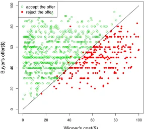
but only 6 out of the 689 offers that exceed the seller’s cost. Clearly, the types of reciprocal behavior and other regarding preferences found pervasive in Ultimatum Bargaining experi-ments are not a factor here. These results also demonstrate the robustness of the findings in Salmon and Wilson (2008).
[image:13.612.154.442.242.499.2]Result 3. Sellers rarely reject profitable offers, and always reject non-profitable ones, con-firming Hypothesis 3.
Figure 4: Plot of take-it-or-leave-it offers versus the auction winning seller’s cost: an open circles marks an accepted offer and a solid circle marks a rejected offer.
● ● ● ● ● ● ● ● ● ● ● ● ● ● ● ● ● ● ● ● ● ● ● ● ● ● ● ● ● ● ● ● ● ● ● ● ● ● ● ● ● ● ● ● ● ● ● ● ● ● ● ● ● ● ● ● ● ● ● ● ● ● ● ● ● ● ● ● ● ● ● ● ● ● ● ● ● ● ● ● ● ● ● ● ● ● ● ● ● ● ● ● ● ● ● ● ● ● ● ● ● ● ● ● ● ● ● ● ● ● ● ● ● ● ● ● ● ● ● ● ● ● ● ● ● ● ● ● ● ● ● ● ● ● ● ● ● ● ● ● ● ● ● ● ● ● ● ● ● ● ● ● ● ● ● ● ● ● ● ● ● ● ● ● ● ● ● ● ● ● ● ● ● ● ● ● ● ● ● ● ● ● ● ● ● ● ● ● ● ● ● ● ● ● ● ● ● ● ● ● ● ● ● ● ● ● ● ● ● ● ● ● ● ● ● ● ● ● ● ● ● ● ● ● ● ● ● ● ● ● ● ● ● ● ● ● ● ● ● ● ● ● ● ● ● ● ● ● ● ● ● ● ● ● ● ● ● ● ● ● ● ● ● ● ● ● ● ● ● ● ● ● ● ● ● ● ● ● ● ● ● ● ● ● ● ● ● ● ● ● ● ● ● ● ● ● ● ● ● ● ● ● ● ● ● ● ● ● ●● ● ● ● ● ● ● ● ● ● ● ● ● ● ● ● ● ● ● ● ● ● ● ● ● ● ● ● ● ● ● ● ● ● ● ● ● ● ● ● ● ● ● ● ● ● ● ● ● ● ● ● ● ● ● ● ● ● ● ● ● ● ● ● ● ● ● ● ● ● ● ● ● ● ● ● ● ● ● ● ● ● ● ● ● ● ● ● ● ● ● ● ● ● ● ● ● ● ● ● ● ● ● ● ● ● ● ● ● ● ● ● ● ● ● ● ● ● ● ● ● ● ● ● ● ● ● ● ● ● ● ● ● ● ● ● ● ● ● ● ● ● ● ● ● ● ● ● ● ● ● ● ● ● ● ● ● ● ● ● ● ● ● ● ● ● ● ● ● ● ● ● ● ● ● ● ● ● ● ● ● ● ● ● ● ● ● ● ● ● ● ● ● ● ● ● ● ● ● ● ● ● ● ● ● ● ● ● ● ● ● ● ● ● ● ● ● ● ● ● ● ● ● ● ● ● ● ● ● ● ● ● ● ● ● ● ● ● ● ● ● ● ● ● ● ● ● ● ● ● ● ● ● ● ● ● ● ● ● ● ● ● ● ● ● ● ● ● ● ● ● ● ● ● ● ● ● ● ● ● ● ● ● ● ● ● ● ● ● ● ● ● ● ● ● ● ●● ● ● ● ● ● ● ● ● ● ● ● ● ● ● ● ● ● ● ●● ● ● ● ● ● ● ● ● ● ● ● ● ● ● ● ● ● ● ● ● ● ● ● ● ● ● ● ● ● ● ● ● ● ● ● ● ● ● ● ● ● ● ● ● ● ● ● ● ● ● ● ● ● ● ● ●
0 20 40 60 80 100
0 20 40 60 80 100 Winner's cost($) Buy er' s off er($) ● ● ● ● ● ● ● ● ● ● ● ● ● ● ● ● ● ● ● ● ● ● ● ● ● ● ● ● ● ● ● ● ● ● ● ● ● ● ● ● ● ● ● ● ● ● ● ● ● ● ● ● ● ● ● ● ● ● ● ● ● ● ● ● ● ● ● ● ● ● ● ● ● ● ● ● ● ● ● ● ● ● ● ● ● ● ● ● ● ● ● ● ● ● ● ● ● ● ● ● ● ● ● ● ● ● ● ● ● ● ● ● ● ● ● ● ● ● ● ● ● ● ● ● ● ● ● ● ● ● ● ● ● ● ● ● ● ● ● ● ● ● ● ● ● ● ● ● ● ● ● ● ● ● ● ● ● ● ● ● ● ● ● ● ● ● ● ● ● ● ● ● ● ● ● ● ● ● ● ● ● ● ● ● ● ● ● ● ● ● ● ● ● ● ● ● ● ● ● ● ● ● ● ● ● ● ● ● ● ● ● ● ● ● ● ● ● ● ● ● ● ● ● ● ● ● ● ● ● ● ● ● ● ● ● ● ● ● ● ● ● ● ● ● ● ● ● ● ● ● ● ● ● ● ● ● ● ● ● ● ● ● ● ● ● ● ● ● ● ● ● ● ● ● ● ● ● ● ● ● ● ●
accept the offer reject the offer
4.3
Buyer behavior
and those above are rejected and countered with an offer on the OOL. Note, we are only plotting a randomly selected one-fourth of the data to avoid over-cluttering.
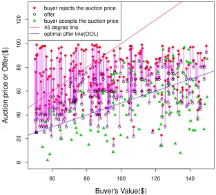
Figure 5: Buyer choices conditional on realized value: accepted auction prices and reject auction prices with counteroffer.
● ● ● ● ● ● ● ● ● ● ● ● ● ● ● ● ● ● ● ● ● ● ● ● ● ● ● ● ● ● ● ● ● ● ● ● ● ● ● ● ● ● ● ● ● ● ● ● ● ● ● ● ● ● ● ● ● ● ● ● ● ● ● ● ● ● ● ● ● ● ● ● ● ● ● ● ● ● ● ● ● ● ● ● ● ● ● ● ● ● ● ● ● ● ● ● ● ● ● ● ● ● ● ● ● ● ● ● ● ● ● ● ● ● ● ● ● ● ● ● ● ● ● ● ● ● ● ● ● ● ● ● ● ● ● ● ● ● ● ● ● ● ● ● ● ● ● ● ● ● ● ● ● ● ● ● ● ● ● ● ● ● ● ● ● ● ● ● ● ● ● ● ● ● ● ● ● ● ● ● ● ● ● ● ● ● ● ● ● ● ● ● ● ● ● ● ● ● ● ● ● ● ● ● ● ● ● ● ● ● ● ● ● ● ● ● ● ● ● ● ● ● ● ● ● ● ● ● ● ● ● ● ● ● ● ● ● ● ● ● ● ● ● ● ● ● ● ●
60 80 100 120 140
0 20 40 60 80 100 120 Buyer's Value($) A uction pr
ice or Off
er($) ● ● ● ● ● ● ● ● ● ● ● ● ● ● ● ● ● ● ● ● ● ● ● ● ● ● ● ● ● ● ● ● ● ● ● ● ● ● ● ● ● ● ● ● ● ● ● ● ● ● ● ● ● ● ● ● ● ● ● ● ● ● ● ● ● ● ● ● ● ● ● ● ● ● ● ● ● ● ● ● ● ● ● ● ● ● ● ● ● ● ● ● ● ● ● ● ● ● ● ● ● ● ● ● ● ● ● ● ● ● ● ● ● ● ● ● ● ● ● ● ● ● ● ● ● ● ● ● ● ● ● ● ● ● ● ● ● ● ● ● ● ● ● ● ● ● ● ● ● ● ● ● ● ● ● ● ● ● ● ● ● ● ● ● ● ● ● ● ● ● ● ● ● ● ● ● ● ● ● ● ● ● ● ● ● ● ● ● ● ● ● ● ● ● ● ● ● ● ● ● ● ● ● ● ● ● ● ● ● ● ● ● ● ● ● ● ● ● ● ● ● ● ● ● ● ● ● ● ● ● ● ● ● ● ● ● ● ● ● ● ● ● ● ● ● ● ● ● ● ●
buyer rejects the auction price offer
buyer accepts the auction price 45 degree line
optimal offer line(OOL)
The figure suggests mixed evidence regarding how theory does track the data. Buyers reject 82% of the auction prices above the OOL, and accept 74% of those below the OOL; roughly matching the theoretical predictions. However, we can recognize there are three types of behavior which deviate the theoretical prediction. First, we observe that when some high auction prices are rejected, the subsequent counteroffer is greater than the theoretical optimal offer. Second, some auction prices above the OOL are accepted. Third, some behavior is more aggressive that theory predicts; some counteroffers are below the OOL and even some auction prices below the OOL are rejected. Are these deviations just unbiased noisy adoption of equilibrium strategies, or is there systematic structure driven by alternative behavioral features?
simply accepts the auction price and purchases with probability one.) Formally, the Tobit model is
oit=
α+βpit+γvit+ǫit, if α+βpit+γvit+ǫit < pit
pit, if α+βpit+γvit+ǫit ≥pit
, (4)
where ǫit is a normally distributed error term, N(0, σǫ2).
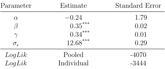
[image:15.612.165.447.275.394.2]If buyers follow the optimal strategy, given in Equation (1), then we should find α=β = 0, and γ = 0.5. We report the maximum likelihood estimates of Equation (4) in Table 3.8
Table 3: MLE of the linear Tobit model for the pooled data
Parameter Estimate Standard Error
α −0.24 1.79
β 0.35*** 0.02
γ 0.34*** 0.01
σǫ 12.68*** 0.29
LogLik Pooled -4070
LogLik Individual -3444
***Coefficient is significant at the 1% level.
The Tobit regression results in Table 3 reveals that the theory does a remarkably good job of predicting when a buyer chooses to bargain, but fails to capture important aspects of what determines the size of take-it-or-leave-it offers. First, we expect a buyer to bargain when
α+γ
1−βv < p. We find that α is not significant and then by substituting parameter estimates forγ andβ, we estimate the condition for choosing to bargain condition is 0.34
1−0.35v = 0.52v <
p; almost exactly what the theory predicts. However, inconsistent with the theoretical prediction is the significant positive relationship price has on the take-it-or-leave-it offer amount. We seek to explain this systematic deviation from the theory.
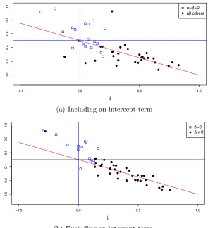
First, we identify significant individual heterogeneity in the buyers’ sensitivities to price. We estimate a separate a individual linear tobit model for each buyer and report the sum of individual Log-likelihood values, in the last row of Table 3. A likelihood ratio test soundly rejects the pooled model in favor of the individual model. In Figure 6 we present scatter plots of the estimated individual coefficients including and excluding the intercept term.
8Out of concern that buyers use one rule to determine when to bargain and another to determine the
These scatter plots of individual estimated pairs β and γ demonstrate that individuals generally agree on when to bargain, but differ in how strong counter offers depend upon the auction price. We provide a vertical reference line at β = 0 and a horizontal reference line at γ = 0.5. The line with a slope of negative one-half passing through (0,0.5) repre-sents the pairs of parameter values corresponding to the rule of negotiating when p >0.5v. South-eastern movements along this line, away from (0,0.5), indicate counteroffers with an increasing positive relationship with auction price. We separate individuals into those whose offers depend upon price, identifying them with solid circles, and those whose offers don’t, identifying them with open squares. The distribution of estimated parameter pairs are clus-tered around the theoretical line for rejection of the auction price but spanning a large range of price sensitivity of counter offers. A natural question is whether these dependencies of take-it-or-leave-it offers on auction prices are consistent with less restrictive assumptions on subject preferences or formation of beliefs.
Figure 6: Individual estimated price and value coefficients from the linear Tobit model
−0.5 0.0 0.5 1.0
0.0
0.2
0.4
0.6
0.8
1.0
β
γ
● ●●
● ●
● ● ●
● ● ●
● ● ● ●
● ●
●
● ●
● ● ●
● ●
●
●
●
●
●
α=β=0
all others
(a) Including an intercept term
−0.5 0.0 0.5 1.0
0.0
0.2
0.4
0.6
0.8
1.0
β
γ
● ●
● ●
● ● ●
● ●
●
●
● ●
● ●
● ● ● ●
●
● ●
● ●
● ●
●
● ●
●
● ● ●
● ●
●
β=0
β ≠0
5
Alternative models
In this section we explain buyer behavior by supposing posterior beliefs regarding the auction winner’s cost are distortions of the Baye’s rule determined posteriors. We parameterize these distortions using a well known probability weighting function that allows an interpretation of subjects perceiving various kinds of affiliation between the lowest and second lowest realized costs. We also show the observed patterns of when buyers choose to bargain and the positive relationship between take-it-or-leave-it offers and auction price can’t be explained by models assuming risk aversion or anticipated regret, models that have previously success explaining empirical auction behavior.
5.1
Subjective posteriors: a probability weighting approach
We previously showed that the invariance of the buyer’s optimal offer depends on the use of Bayes’ Rule to formulate the posterior distribution of the auction winning seller’s cost. We now generalize from Bayesian updating by using a two-parameter transformation of Bayesian posteriors. Namely, the buyer’s subjective posterior of the winner seller’s cost is
G(o|p) =
0 if o= 0
e−µ(−ln(FF((op))))
λ
if 0< o≤p
, (5)
where µand λ >0.
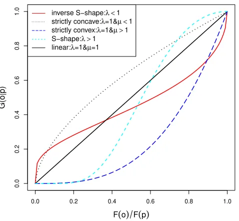
Readers may recognize that Equation (5) is the Prelec (1998) form of a probability weighting function. Probability weighting is a component of Prospect Theory (Kahneman and Tversky, 1979) capturing the empirical regularity that individuals’ valuation of a risky prospect is more sensitive to changes in probabilities close to zero and one than more central quantiles. This common pattern of valuation results in an inverted S-shape probability weighting function. Since we are modeling distorted posteriors we adopt the Prelec form which allows various forms of biases. Using our uniform prior, for example, the unbiased transformation of the Bayesian posterior is the linear G(o|p) presented in Figure 7. Now consider the short-dashed S-shaped G(o|p) in the same figure. In this case, the bias reflects a single-peaked posterior PDF with a subjective expectation that the winner’s cost is about 60% of the auction price; essentially perceiving a non-existent affiliation in cost. A stronger bias towards a positive affiliation in cost is found in the convex shaped G(o|p), while a concave G(o|p) suggests a bias in favor of low costs.9 In this case the subjective posterior
9Whenλ = 1 this model is behavioral indistinguishable from a model of a buyer whose expected
puts increasing probability mass nearer the auction price. Let’s finally consider the inverted S-shaped G(o|p) which implies increasing posterior beliefs on costs close to zero and the price. This suggests a rather unusual u-shaped posterior PDF.
Figure 7: Potential G(o|p)’s generated by the Prelec probability weighting function
0.0 0.2 0.4 0.6 0.8 1.0
0.0
0.2
0.4
0.6
0.8
1.0
F(o) F(p)
G(o|p)
inverse S−shape:λ <1 strictly concave:λ=1&µ <1 strictly convex:λ=1&µ >1 S−shape:λ >1 linear:λ=1&µ=1
Now suppose a buyer formulates his posterior distribution of the auction winner’s cost according to Equation (5). The next proposition describes when there is a unique optimal offer, and under what conditions an interior optimal offer is strictly increasing in price.
Proposition 2. AssumingF(c)is the uniform distribution andG(o|p)is calculated according to Equation (5), then
(i) if λ≥1 and f′(o)≤0, then o+G(o|p)
g(o|p) is strictly increasing and there is a unique o ∗;
(ii) if λ >1, then an interior optimal offer o∗ is strictly increasing in the auction price p.
Proof: See appendix.
A buyer’s Nash equilibrium strategy, when following our two parameter subjective pos-terior model, directly leads to the following non-linear Tobit regression model;
oit =
o∗
it(µ, λ|pit, vit) +ǫit, if o∗it(µ, λ|pit, vit) +ǫit< pit
pit, if o∗
it(µ, λ|pit, vit) +ǫit≥pit
Z(v−o)FF((Po))µ = (v−o)µ1 F(o)
F(P), where Z(y) = y
1
µ. We refer the reader to Goeree, Holt, and
where ǫit is a normally distributed error term, N(0, σ2ǫ), ando∗it(µ, λ|pit, vit) comes from the first order condition v−o∗ = G(o∗|p)
g(o∗|p).
According to Amemiya (1984), The likelihood function of the non-linear Tobit model is,
max
µ,λ L(µ, λ, σ
2|o, v, p) = 48
Y
i=1 30
Y
t=1
Y
pit≤oit
Pr(o∗it ≥pit) Y pit>oit
f(oit|o∗it < pit) Pr(o
∗
it < pit).
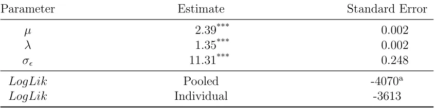
Table 4 reports the maximum likelihood estimation results of this nonlinear Tobit model. The estimates ofµ= 2.39 andλ= 1.35 imply thatG(o|p) is s-shaped and there is a positive relationship between the offers and auction prices.10 A Wald test rejects the Bayesian model,
µ = λ = 1, in favor of this subjective prior model with a p-value of less than 0.001. Once again there is significant heterogeneity across individuals as a full fixed coefficient model can’t be rejected with a likelihood ratio test (see the last row of Table 4 for the Log-likelihood value of the fixed coefficient regression.)
The fixed coefficient model exhibits a diversity of behavioral rules which we now connect to the individual estimates of the structural parametersµandλ. First, we present in Figure 8 a scatter plot of each buyer’s joint estimate of (µi, λi). We classify each buyer’s subjective posterior function according to the following joint hypothesis tests.11
1. Linear - we fail to reject µ=λ= 1.
2. S-shaped - we reject λ = 1 in favor ofλ >1.
3. Inverted s-shaped - we reject λ= 1 in favor of λ <1.
4. Strictly convex - we fail to reject λ = 1 and we rejectµ= 1 in favor ofµ > 1. 5. Strictly concave - we fail to reject λ= 1 and we reject µ= 1 in favor of µ <1.
Let’s consider four subjects with differing shaped subjective posterior functions, and compare how the shape of the function corresponds to their behavior in the experiment. First, consider Buyer A whose parameter estimates are marked “A” in Figure 8 and close to the Bayesian type at (1,1). Buyer A’s estimated G(o|p) and his choice data are presented in the first row of plots of Figure 9. Here we see that his subjective posterior transformation is nearly one-to-one with the Bayesian posterior, and correspondingly his experimental choices of when to bargain and consequent take-it-or-leave-it offers closely agree with the theory. Buyer B, in contrast, has a s-shaped subjective posterior consistent with a disproportionately high perception that the auction winner’s cost be between 20-80% of the auction price. This leads Buyer B to reject every auction outcome and make aggressive counter offers. Buyer
10Finding probability weighting functions that are not inverted s-shaped is common in strategic decision
tasks; for example bidders in first price sealed bid auctions have been estimated to have convex shaped functions (Goeree, Holt, and Palfrey, 2002; Ratan, 2012) and s-shaped in normal form games (Goeree, Holt, and Palfrey, 2003).
Table 4: MLE of the non-linear Tobit model with the two parameter subjective posterior model
Parameter Estimate Standard Error
µ 2.39*** 0.002
λ 1.35*** 0.002
σǫ 11.31*** 0.248
LogLik Pooled -4070a
LogLik Individual -3613
***Coefficient is significant at the 1% level.
a This is not a typo, this is the same value for the maximized likelihood as we find for the linear
Tobit model. However, the linear Tobit model has one more parameter than the nonlinear Tobit model.
C’s posterior reflects a different belief of affiliation; the convex posterior reflects a belief the winner’s cost is very likely close to the auction price.12 Consequently, the buyer seldom
rejects the auction outcome and demands very small price reductions in the few cases he does. On the other end of the optimism spectrum, is Buyer D whose concave posterior function that exhibits a strong negative bias on the winners cost, and leads to a high rejection rate and very aggressive counteroffers.
5.2
Risk aversion and anticipated regret: two (non)explanations
Two behavioral models successfully used to explain bidder deviations from Nash equilibrium strategies are risk aversion (Cox, Roberson, and Smith, 1982; Cox, Smith, and Walker, 1988) and anticipated regret (Engelbrecht-Wiggans and Katok, 2007, 2009; Filiz-Ozbay and Ozbay, 2007). However, neither model can explain the positive relationship between auction prices and take-it-or-leave offers. Risk aversion alone can only influence the location of the optimal offer line. While in the case of anticipated loss regret, there is no impact on the buyer’s strategy when the auction price exceeds his value and there is a negative relationship between take-it-or-leave-it offers and auction price when his value exceeds the auction price. First consider the case where the buyer is strictly risk averse but forms Bayesian poste-riors. For our experimental setting the following proposition shows that for any v the the optimal take-it-or-leave-it offer exceeds the risk neutral case and the amount of this offer does not vary with price.
12The reader may notice that we estimate seven buyers having inverted s-shapedG(o|p); however, in each
Figure 8: Individual estimates of parameters µand λ from the subjective posterior model
0 2 4 6 8
0.0
0.5
1.0
1.5
2.0
2.5
µ
λ
●
● ●
●●
● ●
● ●
● ●
● ●
●
A B
C D
● strictly convex S−shape strictly concave ● linear inverse S−shape
Proposition 3. Assume the buyer’s expected utility function satisfies u(0) = 0, u′(x) > 0,
and u′′(x)<0, then
(i) the optimal offer o∗ is greater than the optimal offer for the risk neutral case.
(ii) For an interior optimal offer o∗, ∂o∗
∂p = 0.
Proof: See appendix.
Consider an example in which a buyer in our experiment has the expected utility function
u(x) =xr, characterized by the constant coefficient of relative risk aversion r. For a strictly positive r, the buyer’s Nash equilibrium strategy is to accept all auction prices below the thresholdo∗(v;r) and to counter offer this threshold otherwise. It is straight forward to show
that o∗(v;r) = v
1+r. In Figure 10, the left hand side plot shows the hypothetical behavior of a buyer for whom r = 0.5. Clearly the offers don’t depend upon the price and OOL is steeper than the risk neutral case.
Figure 9: Four different estimatedG(o|p) and the corresponding buyer subject behavior
●
●
●
●
●
● ●
● ●
●
● ●
● ●
● ● ●
● ●
60 80 100 120 140
0
20
40
60
80
100
120
A
uction pr
ice or Off
er($)
●
●
●
●
●
● ●
● ●
●
● ●
● ●
● ●
● ●
●
● ●
buyer rejects the auction price offer
buyer accepts the auction price 45 degree line optimal offer line(OOL)
0.0 0.2 0.4 0.6 0.8 1.0
0.0
0.2
0.4
0.6
0.8
1.0
G(o|p)
(a) Buyer A (µ, λ) = (1.05,1.10)
● ●
●
● ●
●
● ●
●
● ●
● ●
●
● ●
●
● ●
●
● ● ●
● ●
● ●
●
● ●
60 80 100 120 140
0
20
40
60
80
100
120
A
uction pr
ice or Off
er($)
● ●
●
●
● ●
● ●
● ● ● ●
●
●
●
●● ● ●●
●
●
●
● ●
● ●
●
● ●
0.0 0.2 0.4 0.6 0.8 1.0
0.0
0.2
0.4
0.6
0.8
1.0
G(o|p)
(b) Buyer B (µ, λ) = (1.28,1.88)
● ●
● ● ●
● ●
● ●
60 80 100 120 140
0
20
40
60
80
100
120
A
uction pr
ice or Off
er($)
● ●
● ● ●
● ●
● ●
0.0 0.2 0.4 0.6 0.8 1.0
0.0
0.2
0.4
0.6
0.8
1.0
G(o|p)
(c) Buyer C (µ, λ) = (6.20,0.96)
● ●
●
●●
● ●
● ●
●
● ● ●
●
●
● ●
●
● ● ●
●
60 80 100 120 140
0
20
40
60
80
100
120
Buyer's Value($)
A
uction pr
ice or Off
er($)
● ●●
●● ●
● ●
●
●
● ●
●
● ●
●
●
●
● ●
●
●
0.0 0.2 0.4 0.6 0.8 1.0
0.0
0.2
0.4
0.6
0.8
1.0
F(o)F(p)
G(o|p)
accepted. In this case the magnitude of the win regret is unknown, unlike the case of loss regret. Here we will follow the suggestion of Davis, Katok, and Kwasnica (2011) and set the win regret equal to the accepted offer less the expected winner seller’s cost conditional on this bargaining outcome; namely o
2. 13
Let’s consider an explicit model in which win and loss regrets result in decrements to utility by proportional penalties ωw and ωl respectively. In this case we can express the expected utility of an offer o as
E[u(o|v, p;ωw, ωl)] =
v−o 1 + ωw2 o
p −ωl(v−p)
1− op if p < v
v−o 1 + ωw
2
o
p if p≥v
. (6)
Conditional upon bargaining, the optimal take-it-or-leave-it offer is
o∗(v, p,;ωw, ωl)] =
v+ωl(v−p)
2(1+ωw
2 )
if p < v
v
2(1+ωw
2 )
if p≥v . (7)
From Equation (7) when the auction price exceeds the buyer’s value, his optimal offer does not depend upon the auction price. When price is below his value, then there exists a negative relationship which is the opposite of what we observe. When deciding whether to bargain, the buyer evaluates whether v −p exceeds his expected utility (6) evaluated at his optimal offer given in Equation (7). We present the hypothetical decisions of a buyer for whom ωw = 0 andωl = 0.5 on the right hand side of Figure 10.
13We proceed assuming there is no winner’s regret for accepting the auction outcome, doing so only
Figure 10: Buyer behavior under risk aversion and anticipated regret: some hypothetical decisions for randomly selected decision scenarios
● ● ● ● ● ● ● ● ● ● ● ● ● ● ● ● ● ● ● ● ● ● ● ● ● ● ● ● ● ● ● ● ● ● ● ● ● ● ● ● ● ● ● ● ● ● ● ● ● ● ● ● ● ● ● ●● ● ● ● ● ● ● ● ● ● ● ● ● ● ● ● ● ● ● ● ● ●● ● ● ● ● ● ● ● ● ● ● ● ● ● ● ● ● ● ● ● ● ●
60 80 100 120 140
0 20 40 60 80 100 120 Buyer's Value($) A uction pr
ice or Off
er($) ● ● ● ● ● ● ● ● ● ● ● ● ● ● ● ● ●● ● ● ● ● ● ● ● ● ● ●● ● ● ● ● ● ● ● ● ● ● ● ● ● ● ● ● ● ● ● ● ● ●● ● ● ● ●● ● ● ● ● ● ● ● ● ● ● ● ● ● ●● ● ● ● ● ● ●● ● ● ● ● ● ● ● ● ● ● ● ● ● ● ● ● ● ● ● ● ● ● ●
buyer rejects the auction price offer
buyer accepts the auction price 45 degree line
optimal offer line(OOL) risk averse OOL(r=0.5)
(a) Risk averse buyer wherer= 0.5
● ● ● ● ● ● ● ● ● ● ● ● ● ● ● ● ● ● ● ● ● ● ● ● ● ● ● ● ● ● ● ● ● ● ● ● ● ● ● ● ● ● ● ● ● ● ● ● ● ● ● ● ● ● ● ● ● ● ● ●● ● ● ● ● ● ● ● ● ● ● ● ● ● ● ● ● ● ● ● ● ● ● ● ● ● ● ● ● ● ● ● ● ● ● ● ● ● ● ● ● ● ● ● ● ● ● ● ● ● ● ● ● ● ● ● ● ● ● ● ●
60 80 100 120 140
0 20 40 60 80 100 120 Buyer's Value($) A uction pr
ice or Off
er($) ● ● ● ● ● ● ● ● ● ● ● ● ● ● ● ● ● ● ● ● ● ● ● ● ● ● ● ● ● ● ● ● ● ● ● ● ● ● ● ● ● ● ● ● ● ● ● ● ● ● ● ● ● ● ● ● ● ● ● ● ● ● ● ● ● ● ● ● ● ● ● ● ● ● ● ● ● ● ● ● ● ● ● ● ● ● ●● ● ● ● ● ● ● ● ● ● ● ● ● ● ● ● ● ● ● ● ● ● ● ● ● ● ● ● ● ● ● ● ● ● ● ●
buyer rejects the auction price offer
buyer accepts the auction price 45 degree line
optimal offer line(OOL)
(b) Anticipated regret buyer where (ωw, ωl) = (0,0.5)
6
Concluding remarks
In this study we examine behavior in reverse English auctions, followed by a buyer option to engage in ultimatum bargaining. As Bulow and Klemperer (1996) showed, a Nash equi-librium of this game implements the optimal mechanism for procurement. We find strong support for this equilibrium modulo buyer’s ultimatum offers having a positive relationship with auction prices. This turns out to have economic significance as the average buyer’s surplus in our experiment was about 7.5% less than would have been earned with optimal offers. We think these results can benefit supply chain practices. First, it provides justifi-cation for the practice of engaging in post auction negotiations when qualifying additional suppliers is not feasible. Second, it also identifies a particular problem of using the auction information to build accurate beliefs of the winner’s cost in the negotiation phase. Third, we provide an initial model of how decision maker’s form this distorted posterior which can be used to develop corrective measures.
In their experiments, subjects select reserve prices with varying number of bidders.14 While
the optimal reserve is independent of the number of bidders, they find behaviorally there is a strong relationship. In contrast with our results, they find ascribing preferences reflecting anticipated regret provides a better explanation than probability weighting. This raises the question of why different models - one generalizing preferences and the other beliefs - can explain behavior in similar tasks. In our auction-bargaining tasks, accurate posterior beliefs require the buyer to treat the distribution of the winner’s cost conditional on the auction price as though there we simply two sellers no matter how many sellers actually participate in the auction, and then to use Baye’s rule. Our experiment doesn’t vary the number of sellers, and thus we can’t assess this maintained hypothesis. Future experiments making a direct comparison of the two auction formats and varying the number of bidders will hopefully answer the questions, which auction format is better under what conditions, and are the auctioneer’s deviations from his Nash strategy due to preference or belief misspecifications. Sellers who don’t reject strictly profitable offers, no matter how little that profit may be, along with the previous similar finding by Salmon and Wilson (2008) raises interesting questions on the scope of norms of fairness robustly found in ultimatum bargaining conducted in isolation. The obvious open question, do our results arise because of the embedding of the ultimatum game into a competitive market process or because responders “forgive” lopsided proposals due the proposer’s incomplete information? A carefully designed sequence of experiments systematically moving one element at a time from our experimental design to standard ultimatum game experimental design should bring light to this interesting question.
A
Appendix
Proposition 2: AssumingF(c) is the uniform distribution andG(o|p) is calculated accord-ing to Equation (5), then
(i) ifλ≥1 and f′(o)≤0, theno+G(o|p)
g(o|p) is strictly increasing and there is a unique o ∗;
(ii) if λ >1, then an interior optimal offer o∗ is strictly increasing in the auction price p.
Proof: Start by noting the following
g(o|p) = f(o) µλ
F(o)
−lnF(o)
F(p)
λ−1
G(o|p),
and
g′(o|p) =f′(o) µλ
F(o)
−lnF(o)
F(p)
λ−1
G(o|p)−f2(o) µλ
F2(o)
−lnF(o)
F(p)
λ−1
G(o|p)
−(λ−1)f2(o) µλ
F2(o)
−lnF(o)
F(p)
λ−2
G(o|p) +f2(o)µ
2λ2
F2(o)
−lnF(o)
F(p)
2λ−2
G(o|p).
Now the derivative we are interested in is,
d(o+ Gg((oo||pp)))
do = 1 +
g2(o|p)−G(o|p)g′(o|p)
g2(o|p) = 2−
G(o|p)g′(o|p)
g2(o|p) .
Simplifying we get,
d(o+Gg((oo||pp)))
do = 1 +
1
µλ−lnFF((op))λ−1
+ λ−1
µλ−lnFF((op))λ
− f
′(o)
µλf2(o) 1
F(o)
−lnFF((op))λ−1
. (8)
By inspection of Equation (8) we can that our assumption that λ ≥ 1 and f′(o) ≤ 0
ensures this expression is positive.
Next, we substitute for G(o|P) and g(o|P) into Equation (2), the F.O.C for an interior optimal take-it-or-leave-it offer, we have
µλp o∗
−ln
o∗
p
λ−1
= p
v−o∗.
Take ln to both sides,
ln(µλ)−ln(o∗) + (λ−1) ln
−lno
∗
p
+ ln (v−o∗) = 0.
We differentiate with respect to p at the optimal solution to obtain the following:
λ−1 ln(p)−ln(o∗)
1
p−
1
o∗
∂o∗
∂p
− 1
o∗
∂o∗
∂p −
1
v−o∗
∂o∗
∂p = 0. (9)
Rearranging terms we obtain
∂o∗
∂p =
(λ−1) (v−o∗)o∗
vln op∗
+ (λ−1) (v−o∗)
p. (10)
Obviously, the optimal offer should be smaller than the value and larger than the auction price. Hence, when λ >1, ∂o∗
∂p is strictly positive and the optimal offer is strictly increasing in the auction price. Also note that when λ = 1 there is no relationship between optimal offero∗ and auction price p; not surprising as the model becomes observationally equivalent
to assuming the buyer is risk averse/loving utility. Finally, when λ <1, ∂o∗
Proposition 3: Assume the buyer’s expected utility function satisfies u(0) = 0, u′(x)>0,
and u′′(x)<0, then
(i) the optimal offero∗ is greater than the optimal offer for the risk neutral case;
(ii) For an interior optimal offer o∗, ∂o∗
∂p = 0.
Proof: The first order condition for maximization can be expressed
u(v−o∗)f(o
∗)
F(p) −u
′(v−o∗)F(o∗)
F(p) = 0.
Rearranging terms yields
u(v−o∗)
u′(v−o∗) =
F(o∗)
f(o∗). (11)
Letz(x) = uu′((vv−−xx)), then
z′(x) = u(v−x)u
′′(v−x)
u′(v −x)2 −1.
By the strict concavity of u(x),z′(x)<−1.
When o∗ = 0 the left hand side of (11) is strictly positive and the right hand side is zero.
Further, as the left hand side is strictly decreasing and the right hand side increasing, they will intersect at most one time on the domain [0, p]. Since the slope of the left hand side is less than -1 it is decreasing faster than the risk neutral case. Also the utility atu(0) = 0 the same as in the risk neutral case, so u(v)> v. Therefore it will intersect the right hand side higher at a higher offer level than the risk neutral case. Thus, the optimal offer is higher than the risk neutral case.
References
Amemiya, T. (1984): “Tobit models: A survey,” Journal of Econometrics, 24(1-2), 3–61.
Bulow, J., and P. Klemperer (1996): “Auctions versus negotiations,” American Eco-nomic Review, 86(1), 180–94.
Bulow, J., and J. Roberts(1989): “The simple economics of optimal auctions,”Journal of Political Economy, 97(5), 1060–90.
Cooper, D., andE. Dutcher(2011): “The dynamics of responder behavior in ultimatum games: a meta-study,”Experimental Economics, 14(4), 519–546.
Coppinger, V. M., V. L. Smith, and J. A. Titus (1980): “Incentives and behavior in english, dutch and sealed-bid auctions,” Economic Inquiry, 18(1), 1–22.
Cox, J. C., B. Roberson, and V. L. Smith (1982): “Theory and behavior in single object auctions,” in Research in Experimental Economics, ed. by V. L. Smith, vol. 2, pp. 1–43. JAI Press, Greenwich, CT.
Cox, J. C., V. L. Smith, and J. M. Walker (1988): “Theory and Individual Behavior of First-Price Auctions,” Journal of Risk and Uncertainty, 1(1), 61–99.
Croson, R. (1996): “Information in ultimatum games: An experimental study,” Journal of Economic Behavior & Organization, 30(2), 197–212.
David, H. A. (1981): Order Statistics. John Wiley and Sons, Inc., New York, second edn.
Davis, A. M., E. Katok, and A. M. Kwasnica (2011): “Do auctioneers pick optimal reserve prices?,”Management Science, 57(1), 177–192.
Elmaghraby, W. (2007): “Auctions within E-Sourcing Events,” Production and Opera-tions Management, 16(4), 409–422.
Engelbrecht-Wiggans, R., and E. Katok (2007): “Regret in auctions: theory and evidence,”Economic Theory, 33(1), 81–101.
(2009): “A direct test of risk aversion and regret in first price sealed-bid auctions,”
Decision Analysis, 6(2), 75–86.
Filiz-Ozbay, E., and E. Y. Ozbay (2007): “Auctions with Anticipated Regret: Theory and Experiment,” American Economic Review, 97(4), 1407–1418.
Fischbacher, U. (2007): “z-Tree: Zurich toolbox for ready-made economic experiments,”
Experimental Economics, 10(2), 171–178.
Goeree, J. K., C. A. Holt,andT. R. Palfrey(2002): “Quantal Response Equilibrium and Overbidding in Private-Value Auctions,” Journal of Economic Theory, 104(1), 247– 272.
(2003): “Risk averse behavior in generalized matching pennies games,”Games and Economic Behavior, 45(1), 97–113.
Greiner, B. (2004): “An online recruitment system for economic experiments,” in
Forschung und wissenschaftliches Rechnen, ed. by K. Kremer, and V. Macho, vol. 63 of Ges. fur Wiss. Datenverarbeitung, pp. 79–93. GWDG Bericht.