Munich Personal RePEc Archive
Financial Forecast for the Relative
Strength Index
Alfaro, Rodrigo and Sagner, Andres
Central Bank of Chile
April 2010
Online at
https://mpra.ub.uni-muenchen.de/25913/
Financial Forecast for the Relative Strength Index
Rodrigo Alfaro
Central Bank of Chile
Andres Sagner
Central Bank of Chile
April, 2010
Abstract
In this paper we provide a closed-form expression for one of the most popular index in Technical
Analysis: the Relative Strength Index (RSI). Given that we show how the standard binomial
model for the stock price can be used to predict RSI. The algorithm is as simple as to code a
standard European option. In an empirical application to the Chilean exchange rate we show
how the method works having a better out of sample performance than an ARMA(1,1) model.
JEL Codes: E43, G12
Keywords: Relative Strength Index, Binomial Model, Financial Forecast
Corresponding Author: Rodrigo Alfaro, Central Bank of Chile, Agustinas 1180, Piso 2.
Santiago, Chile.
Telephone: (562) 6702791 Fax: (562) 6702464
1
Introduction
It is well-known that traders do not only rely in fundamental analysis to invest in their
port-folios. Indeed, one of the most common tool across them is the use of technical analysis. This
is particular important for developing countries, for example Abarca et al (2007) report that
Chilean traders use technical analysis for investing in the Chilean peso.
In statistical sense this analysis is intended to extract the cyclical component of stock
prices. One simple approach is to compare several moving average measures of the stock price.
Comparing these the analyst is able to “predict” the most probable trend of the stock price.
In this paper we concentrate our effort in the Relative Strength Index (hereafter RSI), which
is defined as the ratio between average-gains over average-gains plus average-losses (Wilder,
1978). To the best of our knowledge this index is very popular among traders, in particular
the ones which portfolios are biased to currencies. We should note that the RSI is available in
most the trader applications and for that the index is given for the traders.
Our first contribution is to derive a closed-form expression for the RSI which acts like
a highly non-linear filter of the stock price. We should note that by definition the index is
between 0 and 100 and for that the analysts say that an asset with RSI outside of the interval
[30,70] is under or overpriced. This rule is based on experience and it will not be discussed in this paper, but it could be analyzed in the same framework that we work here.
The second and more attractive contribution is to provide a “financial forecast” of the index.
For that purpose we use the Binomial Tree Model (BTM) as the distributional assumption for
the stock price. Also the standard Geometric Brownian Motion (GBM) can be used for this
purpose but it requires to use simulations. In order to avoid those computation burden we
provide the asymptotic expansion for the first moment of the RSI which agrees with the BTM.
Given that we believe that the binomial model is a good motivation to show that forecasting
the RSI is similar as pricing a European option.
Finally, we provide an empirical application to the Chilean exchange rate. There we show
how the parameters of the BTM could be calibrated minimizing Mean Squared Error (MSE)
of the one period out-of-sample forecast. Based on daily data we show that the minimum
MSE is obtained by using the last two months of data. This model has a better out-of-sample
2
Modeling the Relative Strength Index
In this section we provide a closed-form expression for the RSI and using standard distribution
for the stock price we show how the expected value of RSI can be computed. For simplicity
we rely on the binomial model, but complex distributions can be analyzed using simulations.
2.1
Working on the definition
For simplicity we consider the unscaled RSI, which implies that the range of this index will be
[0,1]. In particular, letZtbe the RSI for the stock priceSt, and it is defined as
Zt =
At
At+Bt
(1)
whereAtandBtare the average gains and losses up to the the timet. Both are computed as
weighted average, where weights are inversely proportional to the size of the window selected
(K). Usually,K= 13 (RSI-14) but this does not affect the main results of this paper as long asK3 is big enough.
ComponentAtaccumulates average gains, but actually it accumulates non-negative changes,
its definition is based on previous value as:
At =
K K+ 1
At−1+
1
K+ 1(St−St−1) +
, (2)
where ()+is truncated at zero function, which means that (x)+=xifx >0 and zero otherwise.
It is clear that Atwill decrease if stock price is going down. By the same idea, Btis defined
as follows
Bt =
K K+ 1
Bt−1+
1
K+ 1(St−1−St) +
. (3)
Following the previous example,Btwill increase if stock price is going down, as result of this
RSI will decreases. Traders will see this fact as a signal to sell the asset.
Replacing (2) and (3) in (1), and definingφ= 1/K, we have:
Zt =
At−1+φ(St−St−1) + At−1+φ(St−St−1)
+
+Bt−1+φ(St−1−St)
Note that (St−St−1) +
+ (St−1−St) +
=|St−St−1|, where | · |stands for absolute value.
Finally, consider (1 +Rt) =St/St−1, and Xt=St/(At+Bt), then we have
Zt =
Zt−1+φXt−1R +
t
1 +φXt−1|Rt|
. (4)
2.2
RSI meets Binomial Trees and Asymptotic Expansions
With information at timet−1,Ztis a random variable. Note that randomness is generated
bySt. Standard textbooks introduce option valuation using binomial trees (Wilmott, 2007).
This valuation uses a specific distribution for the stock price. That distribution was introduced
in Cox, Ross, and Rubinstein (1979) as an alternative to the Geometric Brownian Motion
proposed in Black and Scholes (1973).
Under this distributional assumption the stock price increases byuif the realized state isH
and decreases bydif the state isL. Following the standard calibration,u >1 andd= 1/u. In addition, the probability of stateH isp, and distribution of the stock price is generated by the combination of these binomial trees. Each combination is defined as step (N). For example, a binomial tree with two steps (N = 2) has the following set of possible paths for the stock price Ω = {HH, HL, LH, LL}. The total number of trajectories are 2N which implies that
for a reasonable size ofN we have enough possible paths to describe any stochastic process. Finally, the probability of eventHH can be computed byp2
.
In terms of RSI, we have four possible values: ZHH
t ,ZtHL,ZtLH, andZtLL. Note thatZtHH
is based onSHH t =u
2
St−1, then
ZHH t =
Zt−1+φXt−1(u 2
−1) 1 +φXt−1(u
2−1) .
ZHL
t andZtLHare based onStHLandSLHt , which are both equal toSt−1, thenZ
HL
t =ZtLH =
Zt−1. Finally,Z
LL
t is based onStLL=d
2
St−1, then
ZLL t =
Zt−1
1 +φXt−1(1−d 2).
Collecting the previous results we note that the expected value ofZtwith information at time
Et−1(Zt) = p2ZtHH+p(1−p)Z HL
t + (1−p)pZ LH
t + (1−p)
2 ZLL
t
= p2
Z
t−1+φXt−1(u 2
−1) 1 +φXt−1(u
2−1)
+ 2p(1−p)Zt−1+ (1−p) 2
Z
t−1
1 +φXt−1(1−d 2)
.
In order to understand the previous formula consider an Taylor approximation ofd2
aroundu2 0,
this meansd2
= (1/u2
0)−(1/u 4 0)(u
2
−u2 0) +O(u
4
). Evaluating atu0= 1 we haved2
≈2−u2
.
Using this approximation, we have λt−1 ≡φXt−1(u 2
−1) =φXt−1(1−d 2
), taking this and
having statesH andLwith equal probabilities (p= 1/2) we have
Et−1(Zt) ≈
1 4
Z
t−1+λt−1
1 +λt−1
+ 2Zt−1+ Zt−1
1 +λt−1
= 1 2
Z t−1
1 +λt−1
+1 2Zt−1+
1 4
λ t−1
1 +λt−1
= Zt−1+
1 2
λ t−1
1 +λt−1
1 2−Zt−1
.
Note that λt−1 > 0 by definition, then Zt−1 returns to one half. This makes the index
stationary around that level. However, the stock price is a martingale.
Et−1(St) = p 2
SHH
t + 2p(1−p)S HL
t + (1−p)
2 SLL t = u2
+ 2 +d2
4
St−1≈St−1
Note that if St is a martingale then simple averages preserve that property. In statistical
terms, the stock price will have a unit root meanwhileZtis expected to be stationary. In fact,
Ztwill be a martingale whenu= 1 which implies thatσ= 0. In practical terms,Ztis suitable
to be modeled by a standard ARMA process, as we do in the following section.
Noting that expected value of RSI is similar as the price of a European option, we have a
closed form solution (van der Hoek and Elliot, 2000):
Et−1(Zt) =
N X i=0
N!
i!(N−i)!p
i(1
−p)N−i
"
Zt−1+φXt−1 u 2i−N
−1+
1 +φXt−1|u2i−N −1|
#
(5)
where the estimators for probabilitypand factorsuand dcan be obtained by matching the moments of the binomial distribution with the moments of the stock returns. Following the
standard approach (Wilmott, 2007) we could consider a binomial tree with N steps, and let
d= 1/uandp= (a−d)/(u−d) wherea= exp(µ/N).
Note that (5) provides a “financial forecast” based on the distributional assumption of stock
price. Given that binomial distribution is a standard assumption in option pricing it seems
fair to use it for this purpose. However, some traders may disagree about this distribution.
For that reason, we introduce a asymptotic expansion of the variableZt in terms of the size
of the window (K).
Asymptotic expansions are useful tools in econometrics and can be used to derived
ap-proximation of the moments of unknown distributions. In this context, there is three methods
to approximate the moments of a unknown distribution: Laplace, Nagar, and Kadane (Ullah,
2004). Here, we use Nagar expansion which is based on terms of the sample size, here the size
of the window. The asymptotic expansion relies in a bigK (or smallφ). Note that
1 1 +φXt−1|Rt|
= 1−φXt−1|Rt|+φ2Xt2−1R 2
t+Op(φ3).
Replacing this into the formula of RSI, we have
Zt ≈ Zt−1+φXt−1R+t
1−φXt−1|Rt|+φ2Xt2−1R 2
t
= Zt−1+φXt−1 R +
t −Zt−1|Rt|
+φ2 X2
t−1 Zt−1R 2
t−R
+
t|Rt|
This equation can be used for any distributional assumption of the stock price. For example,
consider the expansion up to Op(φ2) and the standard Geometric Brownian Motion as
dis-tributional assumption. Wilmott (2007) provides a simple approximation for the value of an
option when it is at the money (K =St−1e
r) which is E
t−1[(St−K) +
] ≈0.39St−1σ. With
that we have: Et−1(R +
t) = (1/St−1)Et−1[(St−St−1) +
] ≈0.39σ, and by the same argument
Et−1(|Rt|) = 0.78σ, then the expected value of RSI is
Et−1(Zt) =Zt−1+ 0.78φσXt−1
1
2 −Zt−1
+O φ2
. (6)
We can compare this result with the one obtained by the binomial model using N = 2. In both cases RSI returns to its stationary value one half, and the size of the perturbation is
3
Empirical Application: the case of CLP
Abarca et al (2007) report than the RSI is widely used by Chilean analyst that trades in
dollars. In this section we provide the empirical results of applying the financial forecast
proposal using the Binomial Tree Model (BTM) for the underlying process. For the whole
sample an ARMA(1,1) fits well the data, however, the BTM provides smaller errors in terms
of the signals.
3.1
Sample Descriptive and ARMA model
For the application of BTM to the CLP we use daily data for the sample June 2000 and April
2009. The daily return and the RSI-14 are summarized in Table 1 in which is possible to
see the increment in volatility after the bankrupcy of Lehman Brothers bank. Indeed, the
standard deviation of daily return in the last part of the sample is about 2.3 times the one
before that date. For the case of RSI-14 we note that unconditional mean is around 1/2 which was expected from the analysis of the previous section. Also, it is interesting to note that
considering the first period, only 20% of sample is in the overpriced/oversold area.
Table 1: Descriptive Statistics
Return
RSI-14
Jun’00-Aug’08
Sep’08-Apr’09
Jun’00-Aug’08
Sep’08-Apr’09
Mean
0.0000
0.0009
0.4933
0.5214
Std Dev.
0.0056
0.0130
0.1470
0.1363
Skewness
0.2775
0.4658
-0.0774
0.4649
Kurtosis
5.5017
4.6185
2.4921
2.3275
P10
-0.0064
-0.0131
0.2983
0.3647
P90
0.0066
0.0155
0.6760
0.7187
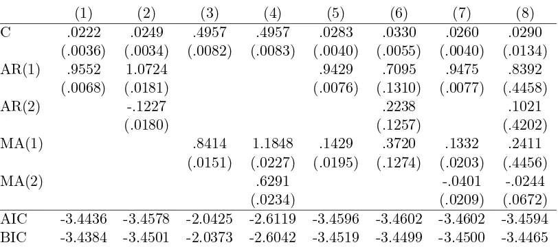
In Table 2 estimations of ARMA models are presented. Using the BIC criteria the
Table 2: ARMA Models of RSI-14
(1)
(2)
(3)
(4)
(5)
(6)
(7)
(8)
C
.0222
.0249
.4957
.4957
.0283
.0330
.0260
.0290
(.0036)
(.0034)
(.0082)
(.0083)
(.0040)
(.0055)
(.0040)
(.0134)
AR(1)
.9552
1.0724
.9429
.7095
.9475
.8392
(.0068)
(.0181)
(.0076)
(.1310)
(.0077)
(.4458)
AR(2)
-.1227
.2238
.1021
(.0180)
(.1257)
(.4202)
MA(1)
.8414
1.1848
.1429
.3720
.1332
.2411
(.0151)
(.0227)
(.0195)
(.1274)
(.0203)
(.4456)
MA(2)
.6291
-.0401
-.0244
(.0234)
(.0209)
(.0672)
AIC
-3.4436
-3.4578
-2.0425
-2.6119
-3.4596
-3.4602
-3.4602
-3.4594
BIC
-3.4384
-3.4501
-2.0373
-2.6042
-3.4519
-3.4499
-3.4500
-3.4465
Standard Errors in parentheses. AIC: Akaike Criteria, and BIC: Schwarz Criteria.
3.2
Implementing the Binomial Tree Model
For simplicity we calibrate the parameters of the binomial model (u and p) using the last
M observations, then we need to minimize a loss function in two dimensions: the size of the window used for the calibration (M) and the number of steps of the tree (N). In this paper we consider 2 loss fuctions: the standard Mean Squared Error (MSE) and a the Mean Change
in sign Error (MCE).
Let ˆZt be the forecast of RSI, ∆ ˆZt= ˆZt−Zˆt−1 its change, and T the sample size, then
M SE = 1
T
T X t=1
(Zt−Zˆt)2 and M CE=
1
T−1
T X t=2
g(∆ ˆZt,∆Zt),
whereg(∆ ˆZt,∆Zt) is one if|∆ ˆZt|/∆ ˆZt6=|∆Zt|/∆Zt, and zero otherwise.
It is clear that MSE will provide a model with more accurate forecasts, meanwhile MCE
will choose a model with less noise in the buy/sell decision of the asset.
Table 3: Grid Search for RSI-14
M
N
5
10
15
20
25
30
35
40
45
10
.2131
.2008
.1968
.1943
.1932
.1929
.1921
.1914
.1925
(.4788)
(.4903)
(.4950)
(.5039)
(.5137)
(.5249)
(.5229)
(.5154)
(.5244)
11
.2125
.2001
.1962
.1937
.1928
.1925
.1918
.1912
.1923
(.4797)
(.4962)
(.4946)
(.5030)
(.5155)
(.5285)
(.5210)
(.5186)
(.5276)
12
.2130
.2007
.1967
.1942
.1932
.1929
.1921
.1914
.1924
(.4801)
(.4903)
(.4959)
(.5043)
(.5137)
(.5221)
(.5215)
(.5177)
(.5257)
13
.2125
.2001
.1962
.1937
.1928
.1925
.1918
.1912
.1923
(.4792)
(.4975)
(.4950)
(.5025)
(.5141)
(.5276)
(.5201)
(.5186)
(.5280)
14
.2129
.2006
.1967
.1941
.1931
.1928
.1921
.1914
.1924
(.4801)
(.4907)
(.4964)
(.5039)
(.5150)
(.5253)
(.5220)
(.5177)
(.5257)
15
.2125
.2001
.1962
.1937
.1928
.1925
.1918
.1912
.1923
(.4792)
(.4975)
(.4941)
(.5020)
(.5141)
(.5276)
(.5192)
(.5186)
(.5280)
16
.2129
.2006
.1966
.1941
.1931
.1928
.1921
.1914
.1924
(.4801)
(.4921)
(.4968)
(.5039)
(.5155)
(.5258)
(.5215)
(.5181)
(.5244)
17
.2125
.2002
.1962
.1937
.1928
.1925
.1918
.1912
.1923
(.4788)
(.4971)
(.4946)
(.5020)
(.5141)
(.5281)
(.5197)
(.5177)
(.5280)
18
.2128
.2006
.1966
.1941
.1931
.1928
.1920
.1914
.1924
(.4801)
(.4930)
(.4964)
(.5020)
(.5155)
(.5258)
(.5215)
(.5177)
(.5248)
19
.2125
.2002
.1962
.1937
.1928
.1926
.1919
.1912
.1923
(.4792)
(.4962)
(.4950)
(.5020)
(.5141)
(.5281)
(.5197)
(.5167)
(.5280)
20
.2128
.2005
.1966
.1940
.1931
.1928
.1920
.1913
.1924
(.4806)
(.4930)
(.4968)
(.5020)
(.5155)
(.5253)
(.5206)
(.5154)
(.5248)
MSE times 10
−3and MCE (in parentheses).
withM up toM = 40 which provides the minimum level, then we have a a minimum MSE at
M = 40 and an oddN. Since we want to have a parsimonius model we pickN= 11.
In terms of MCE we do not observe a decresing or increasing function in withM neither withN. Indeed, the minimum levels of MCE are obtained underM = 5 which means that for this loss function a calibration of the binomial using the lastly data is better than considering
a long period. Again for simplicity we chooseN = 10.
3.3
Out of sample performance
Diebold and Mariano (1995) propose a test to compare the forecasts of two models. This
Table 4: Diebold-Mariano tests for RSI-14
z-value
p-value
d
KEC
0.210
0.833
d
KES
-1.719
0.086
ARMA(1,1) model using two loss functions: MSE and MCE. The BTM model uses N = 10 and M = 5 meanwhile the ARMA(1,1) is estimated using windows of 300 observations. For the estimation of the standard errors of the Diebold-Mariano test we use the information of
the partial autocorrelogram of the difference between forecast errors. Empirically, we note
that MCE requires one lag for the estimation of a robust variance, meanwhile MSE does not
need to include additional lags.
The results (non reported) show that using the MSE measure both BTM and ARMA(1,1)
have the same forecast error, since there is not a significant difference between them. However,
using the MCE measure the BTM model has a lower error than the ARMA model.
4
Conclusions
In this paper, we provide a closed-form expression for the Relative Strength Index (RSI),
which is a popular index in Technical Analysis. Using that definition we show that a forecast
of the Relative Strength Index (RSI) can be obtained by using the standard option valuation
tools. Indeed, under the binomial model is easy to prove that RSI is stationary around its
unconditional mean (one half).
Given that we use the valuation model for forecasting we call our approach “financial
fore-cast”. It is important to stress that underlying model is indeed consistent with many financial
contracts, and for that the use in forecasting opens an opportunity. Using the Chilean
ex-change rate as empirical application we show that our financial forecast, based on the Binomial
Tree Model (BTM) provides a similar Mean Squared Error than modelling the RSI-14 using
the standard time-series approach (ARMA processes). However, in terms of the signals the
References
Abarca, A., F. Alarcon, Pincheira, P. and J. Selaive (2007) “Nominal Exchange Rate in Chile: Predictions Based on Technical Analysis,”Journal Economia Chilena, Banco Central de Chile, 10(2): 57-80.
Black, F., and M., Scholes (1973) “The Pricing of Options and Corporate Liabilities,”Journal of Political Economy, 81:637-659.
Cox, J., S. Ross, and M., Rubinstein (1979) “Option Pricing: A Simplified Approach,”
Journal of Financial Economics, 7:229-264.
Diebold, F., and X. Mariano (1995) “Comparing Predictive Accuracy.” Journal of Business & Economic Statistics, 13(3): 503-508.
Ullah, A. (2004)Finite Sample Econometrics New York: Oxford University Press.
van der Hoek, J., and R. Elliot (2000) it Binomial Models in Finance. Springer.
Wilder, J. (1978)New Concepts in Technical Trading Systems. Trend Research.