Financialisation Impacting Diversification? Evidence from Indian Equity & Commodity Markets

(1)

http://www.scirp.org/journal/tel ISSN Online: 2162-2086 ISSN Print: 2162-2078

Financialisation Impacting Diversification?

Evidence from Indian Equity &

Commodity Markets

Siddula Narsimhulu

1*

, D. Satish

1

, S. V. Satyanarayana

2

1_{IBS Hyderabad, IFHE University, Hyderabad, India}

2_{Department of Commerce, Osmania University, Hyderabad, India}

Abstract

Investors are constantly looking at diversification of risks by combining equities with other assets in their portfolio. Apart from fixed income securities and real estate re-lated instruments, commodities are also being increasingly used as a portfolio diver-sification strategy. But the overwhelming presence of financial institutions and funds in the commodity markets has resulted in financialisation of commodity markets leading to a greater correlation between equities and commodities especially during recession. This has lead to a reduction in diversification benefits. The paper attempts to study the diversification benefits of investing both in Indian commodities and eq-uities markets in different economic environments using VAR Impulse Response Functions with an aim to find out whether financialization exists. The research found that there was absence of interdependence between the Indian equity and commodi-ties markets which offered a good opportunity for diversification. Also the equicommodi-ties market and commodities market during recession were totally decoupled which showed that the financialization was not present in Indian commodities market and there was a greater scope for diversification during the recession.

Keywords

Diversification, Financialisation, Impulse Response Function, Commodities, Recession, Comdex, Nifty

1. Introduction

Diversification has always been an important motive behind construction of portfolios. Traditionally, equity portfolios were built with low or negatively correlated stocks. But How to cite this paper: Narsimhulu, S.,

Satish, D. and Satyanarayana, S.V. (2016) Financialisation Impacting Diversification? Evidence from Indian Equity & Commodity Markets. Theoretical Economics Letters, 6, 837-853.

http://dx.doi.org/10.4236/tel.2016.65088 Received: July 22, 2016

Accepted: September 3, 2016 Published: September 6, 2016

http://creativecommons.org/licenses/by/4.0/

(2)

finding stocks with low correlations became difficult as the economic conditions im-pacted majority of the companies and industries in a similar way. In order to diversify this risk, the investor stated to invest in different economies. But with globalization and liberalization gathering pace, this opportunity for diversification among different equity markets also reduced.

Creating a portfolio of different asset classes was seen as another strategy for diversi-fication. While investing in stocks and bonds is fairly popular, the look for alternate in-vestment intensified in the last couple of years with stocks being combined not only with bonds but also with artifacts, real estates and commodities. Commodities offer a good ground for diversification as they behave distinctly from stocks and bonds. Com- modity prices are not as directly impacted by changes in discount rates as in the case of stocks and bonds. Prices are also not determined by Discounted Cash Flow (DCF) ap-proach but by forces that govern demand and supply for commodities [1].

Inflation has a detrimental effect on stocks and bonds as these lose value with infla-tion. On the other hand, commodities prices are positively related to inflainfla-tion. It is also observed by Dusak [2] and Rosansky [3] that commodities prices are impacted by short-term demand and supply expectations in the current economy while stocks and bonds are affected by long-term expectations of earnings and coupon rates. Commodi-ties also tend to have positive exposure to event risk. This is because the event risk tends to favor supply disruptions rather than result in sudden increase in supply creat-ing commodity price shocks. These disruptions provide positive returns for commodi-ties while at the same time they provide negative returns for financial assets. Therefore, the event risk associated with commodities tends to favor investors in the commodity markets while detrimentally impacting investors in the financial markets. This is the reason for commodities prices having little or even negative correlation with the prices of capital asset like bonds and stocks.

Commodities markets were existent for a long time, but absence of liquidity, physical delivery and counterparty risks hindered investment in commodities. With the coming of the commodities exchanges not only the risk is shifted to the clearing houses but also there has been a substantial improvement in liquidity. These developments resulted in increased flow of investment into the commodities market both for making speculative gains as well as to diversify risks. But with the overwhelming presence of financial in-stitutions, pension funds and hedge funds (financialisation) in the commodities market, it was observed that in some markets there has been increased correlation between eq-uity markets and commodities market resulting in commodities losing the alternate in-vestments opportunity especially during recession [4].

(3)

2. Review of Literature

Research into whether commodities can be used as an asset class in a portfolio context is being done for quite some time. Ankrim, Ernest M; Hensel, Chris R [5] in their paper suggests that commodities is a better investment class compared to real estate as in-vesting in commodities not only possessed the typical benefits of real estate but also of-fered the vital liquidity which does not exists in real estate. The paper compares the re-turns of Goldman Sachs Commodity Index (GSCI) and Investible Commodity Index (ICI) with S&P index for a period of 19 years from 1972 to 1990. The paper found that the commodity indices outperformed the stock index in each of the inflationary years. The risk adjusted returns of commodities was higher than stocks for the overall period. They also observed that adding commodities reduced volatility of returns more than the reduction of returns.

In a research paper studying the relationships between stocks and commodities writ-ten by Richard Keary and David Stanbridge [6] showed the benefits of investing in un-leveraged passive long term investment in commodity futures. The paper also showed that adding commodities in a portfolio of stocks would offer diversification. The paper analyzed risk, return and correlation statistics of traditional benchmarks with com-modity indices and a typical balanced portfolio in Australian markets. The data studied was for 3 year, 5 year and 10 years period respectively. Though the risk and return sta-tistics were not interesting the correlation of the commodity indices with the traditional assets were very low and negative for some periods.

Bahattin, et al. [7] attempted to study the extent to which commodity and equity prices and returns were in synchrony and also to know whether the intensity of the co movements increased over time. S&P 500 and DJIA Index were used as proxy for equity and DJ AIG and GSCI index was taken as proxy for Commodities. Data was taken for 17 years from 1991 to 20018. The author used GAARCH Model to estimate the time varying variances and then the standardized residuals from this estimation was used to come up with time varying correlation matrix. To estimate the long term relationship Johnson Co-integration analysis was used. The study found a no persistent increase in co movements between equities and commodities in the period of the study. The study concluded that commodities can often provide benefits in terms of portfolio diversifi-cation.

Akash Dania [8] in the paper studied the nature of the relationship between com-modity and stock markets. Vector Auto Regression (VAR) was used to study the inter-dependencies between Precious Metals, Industrial Metals, Agriculture Produce and eq-uity market returns. Data between January 1990 and April 2008 was taken and S&P 500 returns were taken as a proxy for performance of equity market. Results suggested commodity market returns and equity market returns have little or no significant posi-tive interdependence, thereby signaling diversification benefits from investing in the commodity sector.

(4)

between the two asset classes were less or near zero before the 2008 financial crises but increased during the crises, showing that commodities lost the alternate asset class sta-tus. The author concluded that increased financialization (overwhelming presence of financial institutions, pension funds and hedge funds) of the Japanese commodity markets with many financial institutions having exposure to the market has increased the correlation between stocks and commodities.

Radosław Kurach [9] in the paper analyzed diversification benefits by investing in commodities from a polish investor point of view by converting all the US Dollar re-turns into Polish Currency. The authors analyzed dependence structure between Pol-and (PL) Pol-and some regional indices, namely: World (WRD), Emerging Markets Asia (EMA), Emerging Markets Europe (EME) and BRIC (Brazil, Russia, India, and China). As a proxy of the broad commodity exposure, Standard & Poors Total Return Goldman Sachs Commodity Index (GSCI) was taken. The paper found that there was little corre-lation between commodities and stocks and after converting into the local currency the degree of co movement decreased further, increasing the chance for diversification.

Hector O. Zapata, Joshua D. Detre, and Tatsuya Hanabuchi [10] worked on stock market and commodities data from 1971 to 2011 to study the historical relationships. The study found that there was a negative correlation between stock and commodities for the period and stocks and commodities in US have alternated in price leadership with cycles of 29 to 32 years. The authors also found that portfolio allocation by a risk-averse investor, irrespective of the period analyzed, placing funds in agribusiness and/or agricultural commodity indexes was a good investment decision. The analysis was done using MOTAD and Target MOTAD linear programming model was used.

Yu-Min Wang, Chia-Fei Lin and Yu-Hsien Li [11] in their research studied the cor-relation between commodities and stocks. Commodity market indices were divided in-to the four categories of composite commodities, agricultural commodities, energy, and metals. Data was gathered from 12 countries from period January 31st 2005 to February 17th 2012. This study analyzed the role that the characteristics of these four commodity indices play in stock-market investment portfolio strategies. This study used a condi-tional volatility ARCH (1) model with a delay of one period as a proxy variable for ab-normal market volatility to examine changes in the returns of the stock and commodity markets. Stable long-term relationships existed between some commodity and stock markets, and that commodity indices generally lead stock market indices during serious crises or during high volatility in stock markets. Under normal stock market circums-tances, no hedging effects existed between commodity market indices and stock mar-kets.

(5)

on a hypothetical portfolio of historical data which found that long-term commodity investment provided a small benefit as a defensive asset due to its low correlation with US equities. However, the diversification benefit from commodity investment de-pended on the commodities selected.

Saban Nazlioglu et al. [13] have examined volatility transmission between oil and se-lected agricultural commodity prices (wheat, corn, soybeans, and sugar). They have ap-plyed the newly developed causality in variance test and impulse response functions to daily data from 01 January 1986 to 21 March 2011. In order to identify the impact of the food price crisis, the data are divided into two sub-periods: the pre-crisis period (01 January 1986 to 31 December 2005) and the post-crisis period (01 January 2006–21 March 2011). They found out that there is no risk transmission between oil and agri-cultural commodity markets in the pre-crisis period, oil market volatility spills on the agricultural markets—with the exception of sugar—in the post-crisis period. The im-pulse response analysis also indicated that a shock to oil price volatility is transmitted to agricultural markets only in the post-crisis period. This study thereby has shown that the dynamics of volatility transmission changes significantly following the food price crisis. After the crisis, risk transmission emerges as another dimension of the dynamic interrelationships between energy and agricultural markets.

Walid Mensi [14] employed a VAR-GARCH model to investigate the return links and volatility transmission between the S&P 500 and commodity price indices for energy, food, gold and beverages over the turbulent period from 2000 to 2011. For re-turn and volatility spillover, the results showed significant transmission among the S&P 500 and commodity markets. The authors analyzed the optimal weights and hedge ra-tios for commodities and S&P 500 portfolio holdings using the estimates for each index. The past shocks and volatility of the S&P 500 strongly influenced the oil and gold mar-kets. This study found that the highest conditional correlations were between the S&P 500 and gold index and the S P 500 and WTI index.

Fardous Alom [15] in his study investigated the mean and volatility spillover effects of world crude oil prices on the food prices for selected Asia and Pacific countries/areas (viz. Australia, New Zealand, South Korea, Singapore, Hong Kong (China), Chinese Taipei, India and Thailand) by employing vector auto regression (VAR) and genera-lized autoregressive conditional heteroskedasticity (GARCH)-family models over the period 1995-2010. He found that the oil prices positively influence food prices of the selected countries both in mean and in volatility. Stronger mean and volatility spillover effects are found for the recent subsample period suggesting increasing interdepen-dence between world crude oil and Asia-Pacific food markets in recent times. In terms of mean spillover effects net food importer countries’ food price show stronger effects to the shocks, whereas in terms of volatility spillover effects no distinction in absorbing the oil price shocks can be made between exporters and importers. The findings rec-ommend that crude oil prices should be taken into consideration in policy preparation and forecasting purposes for food prices.

(6)

price in South Africa using monthly data covering the period 2002 to 2014. He meas-ured Food price by the South African consumer price index for food while oil price is proxied by the Brent crude oil. The study employed the bivariate GARCH-in-mean VAR model, which allows the investigation of the effect of a negative and positive shock in oil price volatility on food price. The model also allows the oil price uncertainty to be measured as the conditional standard deviation of a one-step-ahead forecast error of the change in oil price. The results have shown that oil price uncertainty has a positive and significant effect on food price in South Africa. And also the responses of food price to a positive and negative oil price shocks is asymmetric.

Coming to the study of the relation between commodities and equities in Indian Context, Y. Bansal et al. [17] examined the role of Indian Commodity Futures as an as-set class in a traditional portfolio consisting of equity and bond for an investor. The paper identified the optimum portfolio mix of all the three assets using Mean variance optimization technique and how the utility of commodity futures changes with the change in risk aversion levels of an investor. The authors found that, on comparing the portfolios with and without commodities, the portfolio with commodities provided an increase in the returns without a corresponding rise in risk. It also provides evidence that with the increase in risk aversion levels of the investor, allocation to commodity future tends to increase.

Commodity market trading over the stock exchange started in India in 2004. Though few research studies have tried to identify the relationship between commodities and equities markets in India, the study of diversification benefits based on different eco-nomic periods (pre-recession, during recession and post-recession) with a view to iden-tify scope for financialisation was not comprehensive. This research would enable us to study the diversification benefits in different scenarios and also most importantly whether this relationship changed in different economic environments and also find whether financialisation existed especially during recession.

3. Data and Research Methodology

3.1. Sources of Data

This research study is done taking data collected from the biggest commodities and stock markets in India-MCX (Multi Commodity Exchange of India) and NSE (National Stock Exchange of India). Daily spot and futures prices of the broad based commodity index at MCX, COMDEX (MCX Composite Commodity Index) and daily spot prices of widely popular and well accepted equity benchmark index on NSE, CNX-NIFTY (NSE all Equity Index) is taken. The exponential daily returns of both these indices are taken for the study.

3.2. Period of the Study

(7)

study into 3 sub periods based on the monthly Index of Industrial Production (IIP) fig-ures taken from India’s central bank, Reserve Bank of India (RBI). Period from June 2005 to March 2008 was considered as pre-recession period. Data from April 2008 to March 2011 was considered as recession period and data from April 2011 to June 2014 was considered as post recession period. The sample had a size of 2230 (N) observa-tions for each of the indices in the study period.

3.3. Research Methodology

The study apples Correlation, Risk-adjusted Returns based on Sharpe Ratio, VAR along with Impulse response functions to study whether diversification benefits changes with changing economic environment.

3.3.1. Testing Stationarity of Daily Returns of CNX Nifty and MCX Comdex Augmented Dickey Fuller (ADF) test is an augmented version of the Dickey-Fuller (DF) test to account for more dynamic specification of the regression of time series models used in DF test. So, ADF test has been employed to analyze the stationarity of Daily Returns of CNX Nifty and MCX Comdex. The following equation describes the estimation of stationarity under ADF test.

0 1

1 p

t t j t j t

j

Y α γY₋ β Y₋ ε

=

∆ = + +

∑

∆ + ₍₁₎

where Yt = RSt and RFt respectively represent daily returns of MCX Comdex and CNX

Nifty at time t. ∆ is the differencing operator, ∆ = −Yt Yt Yt−1. The unit root test is then carried out under the null hypothesis γ = 1 against the alternative hypothesis of γ < 1. Once the value for the test statistic is computed, it can be compared to the relevant critical value for the ADF test. If the test statistic is less than the critical value then the null hypothesis of γ = 1 is rejected and no unit root is present and the series become stationary.

3.3.2. VAR: Impulse Response Functions of CNX Nifty and MCX Comdex

In order to examine the interrelationship and interdependence between CNX Nifty and MCX Comdex returns Vector Auto Regression (VAR) model has been employed. It can successfully capture the simultaneous relation between two time series variables by us-ing their own lagged values. The model to capture the spot and futures returns interde-pendence is as follows:

1 1

p q

St S Si St i Fj Ft j St

i j

R α β R − γ R − ε

= =

= +

∑

+

∑

+ ₍₂₎

1 1

p q

Ft F Fi Ft i Sj St j Ft

i j

R α β R − γ R − ε

= =

= +

∑

+

∑

+ ₍₃₎

where RSt and RFt respectively represent daily returns of MCX Comdex and CNX Nifty.

(8)

[image:8.595.197.552.379.704.2]

4. Data Analysis and Results

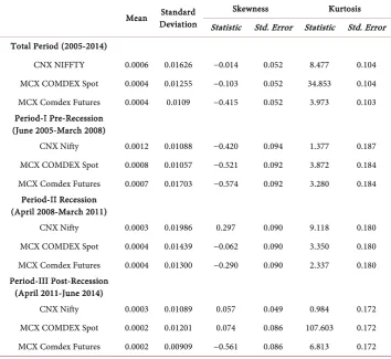
Table 1 reports the descriptive statistics for variables for the period of the sample as well as for each of the sub periods based on the daily returns. The mean daily returns are positive for all the periods. Largely negative skewness was seen indicates a distribu-tion which is asymmetric with tail extending towards negative direcdistribu-tion. Positive skewness was observed in the returns of CNX NIFTY during recession and post reces-sion period. NSE COMDEX spot returns for the post recesreces-sion period also showed skewness with tail extending towards positive direction A Kurtosis figure of greater than 3 was observed for most of the periods with significant peaks for both MCX COMDEX for the total period as well as for the precession period. CNX NIFTY re-turns data in the pre recession and post recession period saw flatter peaks.

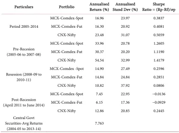
Table 2 shows the returns, standard deviation and Sharpe Ratios. Stock returns ex-ceeded the commodity returns for the period of study with a higher risk .Stocks gave far superior returns in the pre recession period with higher risk but interestingly commod-ities gave better returns during recession with lesser risk. Nifty also gave better returns in the post recession period. Average returns of Indian government bond securities for the period 2004-2014 was taken to calculate the risk–free rate which gave an annual re-turn of 7.69%. Sharpe ratio was less than 1 for the total period with Nifty giving a

Table 1. Descriptive statistics of daily returns of CNX Nifty and MCX comdex.

Mean Standard _Deviation Skewness Kurtosis Statistic Std. Error Statistic Std. Error Total Period (2005-2014)

CNX NIFFTY 0.0006 0.01626 −0.014 0.052 8.477 0.104 MCX COMDEX Spot 0.0004 0.01255 −0.103 0.052 34.853 0.104 MCX Comdex Futures 0.0004 0.0109 −0.415 0.052 3.973 0.103 Period-I Pre-Recession

(June 2005-March 2008)

CNX Nifty 0.0012 0.01088 −0.420 0.094 1.377 0.187 MCX COMDEX Spot 0.0008 0.01057 −0.521 0.092 3.872 0.184 MCX Comdex Futures 0.0007 0.01703 −0.574 0.092 3.280 0.184

Period-II Recession (April 2008-March 2011)

CNX Nifty 0.0003 0.01986 0.297 0.090 9.118 0.180 MCX COMDEX Spot 0.0004 0.01439 −0.062 0.090 3.350 0.180 MCX Comdex Futures 0.0004 0.01300 −0.290 0.090 2.337 0.180 Period-III Post-Recession

(April 2011-June 2014)

(9)

[image:9.595.193.553.90.358.2]

Table 2. MCX Comdex & CNX Nifty: returns, standard deviations and sharpe ratio.

Particulars Portfolio Annualised _{Return (%)} _{Stand Dev (%)}Annualised _{Ratio = (Rp-Rf)/σp}Sharpe

Period 2005-2014

MCX-Comdex-Spot 16.96 23.97 0.3837 MCX-Comdex-Fut 16.30 20.92 0.4081 CNX-Nifty 23.48 31.07 0.5059

Pre-Recesion (2005-06 to 2007-08)

MCX-Comdex-Spot 33.96 20.78 1.2605 MCX-Comdex-Fut 30.37 20.20 1.1190 CNX-Nifty 54.54 32.99 1.4179

Resession (2008-09 to 2010-11)

MCX-Comdex -Spot 14.90 27.49 0.2596 MCX-Comdex-Fut 14.84 24.84 0.2851 CNX-Nifty 10.82 37.92 0.0806

Post-Recession (April 2011 to June 2014)

MCX-Comdex-Spot 7.45 22.95 −0.0136 MCX-Comdex-Fut 6.15 17.36 −0.0929 CNX-Nifty 12.86 20.85 0.2445 Central Govt

Securities-Avg Returns

(2004-05 to 2013-14) 7.763

better risk adjusted returns compared to COMDEX. Sharpe ratio for both Nifty and COMDEX was greater than 1 in the pre recession period showing good performance with stocks having slightly higher ratio when compared to commodities. In the reces-sion period Sharpe ratio was low with COMDEXs having better ratio compared to Nif-ty. Post recession period saw Nifty having positive Sharpe Ratio, and COMDEX having a negative risk adjusted rate indicating a return less than the benchmark rate.

Table 3 shows Augmented Dickey Fuller (ADF, 1979) and Phillip Perron (PP 1998) unit root test results. In both the tests the null hypothesis is that the series is non-stationary and if the calculated value exceeds the critical value the null hypothesis may be rejected implying the stationary characteristics of the series. In all the series for the total time period of the sample as well as for different sub periods, the calculated value ex-ceeded the critical value at their first difference form (returns) with significance at 1% level, rejecting the null hypothesis of non –stationary.

(10)

[image:10.595.201.554.89.347.2]

Table 3. Testing of stationarity of MCX comdex & CNX nifty returns.

Variables At their first difference (returns) ADF Static PP Static Total Period (June 2005-June 2014)

CNX NIFFTY −44.540* −44.472*

MCX COMDEX Spot −50.008* −50.008*

MCX COMDEX Futures −46.1918* −46.3385* Pre-Recession (June 2005-March 2009)

CNX Nifty −24.77889* −24.73871*

MCX COMDEX Spot −25.15601* −25.15607* MCX COMDEX Futures −27.05994* −27.0862* Recession (April 2008-March 2011)

CNX Nifty −25.63816* −25.63247*

MCX COMDEX Spot −26.73747* −26.76378* MCX COMDEX Futures −25.83236* −25.91985* Post-Recession (April 2011-June 2014)

CNX Nifty −26.0286* −26.0286*

MCX COMDEX Spot −35.5413* −35.6600* MCX COMDEX Futures −27.0656* −27.1725* *Significant at 1% level.

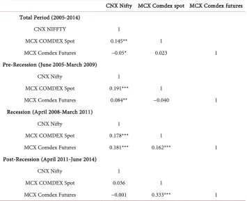
Table 4. MCX comdex & CNX nifty-correlation matrix.

CNX Nifty MCX Comdex spot MCX Comdex futures Total Period (2005-2014)

CNX NIFFTY 1

MCX COMDEX Spot 0.145** 1

MCX Comdex Futures −0.05* 0.023 1

Pre-Recession (June 2005-March 2009)

CNX Nifty 1

MCX COMDEX Spot 0.191*** 1

MCX Comdex Futures 0.084** −0.040 1 Recession (April 2008-March 2011)

CNX Nifty 1

MCX COMDEX Spot 0.178*** 1

MCX Comdex Futures 0.181*** 0.162*** 1 Post-Recession (April 2011-June 2014)

CNX Nifty 1

MCX COMDEX Spot 0.036 1

MCX Comdex Futures −0.001 0.333*** 1

[image:10.595.199.555.392.681.2]

(11)

VAR: Impulse Response Functions of CNX Nifty and MCX Comdex

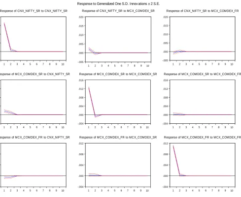
In order to find out, the extent to which the response of one variable respond the shock in another variable, in the short-run a generalized impulse response technique was employed from the VAR model for the total period and also for pre, during and post-recession periods. The optimal lag length in the VAR model was determined by Aikeka Information Criterion (AIC) (refer Annexure I). The impulse response func-tions for one standard deviation shocks in CNX Nifty returns on MCX Comdex Spot and MCX Comdex Futures returns are presented in Figures 1-4 for the total period, pre-recession period, recession and post-recession periods respectively.

[image:11.595.59.549.294.695.2]

The impulse response functions for one standard deviation (S.D) shock (noise) in the CNX Nifty returns on MCX Comdex Spot and Futures are presented in Figure 1 for the Total Period. The results indicate that a shock in the Nifty returns had a positive and significant response on MCX Comdex spot returns for only a period of 3 days and later on diminishes.

Figure 1. Generalized impulse-response functions for the total period. -.005 .000 .005 .010 .015 .020

1 2 3 4 5 6 7 8 9 10

Response of CNX_NIFTY_SR to CNX_NIFTY_SR

-.005 .000 .005 .010 .015 .020

1 2 3 4 5 6 7 8 9 10

Response of CNX_NIFTY_SR to MCX_COMDEX_SR

-.005 .000 .005 .010 .015 .020

1 2 3 4 5 6 7 8 9 10

Response of CNX_NIFTY_SR to MCX_COMDEX_FR

-.004 .000 .004 .008 .012 .016

1 2 3 4 5 6 7 8 9 10

Response of MCX_COMDEX_SR to CNX_NIFTY_SR

-.004 .000 .004 .008 .012 .016

1 2 3 4 5 6 7 8 9 10

Response of MCX_COMDEX_SR to MCX_COMDEX_SR

-.004 .000 .004 .008 .012 .016

1 2 3 4 5 6 7 8 9 10

Response of MCX_COMDEX_SR to MCX_COMDEX_FR

-.004 .000 .004 .008 .012

1 2 3 4 5 6 7 8 9 10

Response of MCX_COMDEX_FR to CNX_NIFTY_SR

-.004 .000 .004 .008 .012

1 2 3 4 5 6 7 8 9 10

Response of MCX_COMDEX_FR to MCX_COMDEX_SR

-.004 .000 .004 .008 .012

1 2 3 4 5 6 7 8 9 10

Response of MCX_COMDEX_FR to MCX_COMDEX_FR

(12)

[image:12.595.112.552.72.380.2] [image:12.595.113.553.390.692.2]

Figure 2. Generalized impulse-response functions for the Pre-recession period.

Figure 3. Generalized impulse-response functions for the recession period. -.005 .000 .005 .010 .015 .020

1 2 3 4 5 6 7 8 9 10

-.005 .000 .005 .010 .015 .020

1 2 3 4 5 6 7 8 9 10

Response of CNX_NIFTY_SR to MCX_COM DEX_SR

-.005 .000 .005 .010 .015 .020

1 2 3 4 5 6 7 8 9 10

-.004 .000 .004 .008 .012

1 2 3 4 5 6 7 8 9 10

-.004 .000 .004 .008 .012

1 2 3 4 5 6 7 8 9 10

-.004 .000 .004 .008 .012

1 2 3 4 5 6 7 8 9 10

-.004 .000 .004 .008 .012

1 2 3 4 5 6 7 8 9 10

-.004 .000 .004 .008 .012

1 2 3 4 5 6 7 8 9 10

-.004 .000 .004 .008 .012

1 2 3 4 5 6 7 8 9 10

Response to Generalized One S.D. Innov ations ± 2 S.E.

-.005 .000 .005 .010 .015 .020 .025

1 2 3 4 5 6 7 8 9 10

-.005 .000 .005 .010 .015 .020 .025

1 2 3 4 5 6 7 8 9 10

-.005 .000 .005 .010 .015 .020 .025

1 2 3 4 5 6 7 8 9 10

-.008 -.004 .000 .004 .008 .012

1 2 3 4 5 6 7 8 9 10

-.008 -.004 .000 .004 .008 .012

1 2 3 4 5 6 7 8 9 10

-.008 -.004 .000 .004 .008 .012

1 2 3 4 5 6 7 8 9 10

-.004 .000 .004 .008 .012 .016

1 2 3 4 5 6 7 8 9 10

-.004 .000 .004 .008 .012 .016

1 2 3 4 5 6 7 8 9 10

-.004 .000 .004 .008 .012 .016

1 2 3 4 5 6 7 8 9 10

(13)

[image:13.595.57.546.76.425.2]

Figure 4. Generalized impulse-response functions for the post-recession period.

The impulse response functions for the pre-recession period are presented in Figure 2. It is observed that there is feedback relationship exists between Nifty and Comdex Spot returns. One standard deviation (S.D) shock (noise) in the CNX Nifty returns is having positive and significant response in MCX Comdex spot returns for about three days and later on becomes insignificant. Also, Nifty spot responded negatively to the shock in Comdex spot but the effect of the shock is dying out in a day.

The impulse response function for the recession period is presented in Figure 3. It is observed that none of the impulse response functions was significant and it implies that Nifty spot and MCX Comdex returns are decoupled.

The impulse response function for the post-recession period is presented in Figure 4. It is observed that negative and significant response on Nifty for one S.D shock to MCX Comdex futures returns and the impact of the shock was observed for about five days and later on becomes insignificant.

5. Findings & Conclusions of the Study

The correlation studies and further VAR results suggest that overall CNX Nifty returns and MCX Comdex returns do not exhibit positive interdependence. During the Pre-

-.004 .000 .004 .008 .012

1 2 3 4 5 6 7 8 9 10

-.004 .000 .004 .008 .012

1 2 3 4 5 6 7 8 9 10

-.004 .000 .004 .008 .012

1 2 3 4 5 6 7 8 9 10

-.008 -.004 .000 .004 .008 .012

1 2 3 4 5 6 7 8 9 10

-.008 -.004 .000 .004 .008 .012

1 2 3 4 5 6 7 8 9 10

-.008 -.004 .000 .004 .008 .012

1 2 3 4 5 6 7 8 9 10

-.002 .000 .002 .004 .006 .008 .010

1 2 3 4 5 6 7 8 9 10

-.002 .000 .002 .004 .006 .008 .010

1 2 3 4 5 6 7 8 9 10

-.002 .000 .002 .004 .006 .008 .010

1 2 3 4 5 6 7 8 9 10

(14)

Recession period though it was observed that Comdex spot responded positively to shock in nifty returns and also the nifty returns responded negatively to shock in the Comdex, but the magnitude and the period of the effect was too small. In the rescission period, the shock in the Nifty returns did not have any impact on the Comdex. During the post recession also the shock in the nifty did not impact Comdex but the shock in the Comdex impacted Nifty but the magnitude was extremely low.

The absence of interdependence between Nifty and Comdex shows that the equity markets and commodities market in India are independent and offer a good opportu-nity for diversification. Also interesting to observe is that the equities market and commodities market during recession were totally decoupled which shows that the fi-nancialisation was not present in Indian commodities market and there was a greater scope for diversification during the recession days. Overall the fund managers with In-dian equities exposure should add commodities in their portfolio to diversify the risk and should increase their exposure to commodities especially during recession.

References

[1] Anson, M.J.P. (2002) Handbook of Alternate Assets. John Wiley & Sons.

[2] Dusak, K. (1973) Futures Trading and Investor Returns: An Investigation of Commodity Market Risk Premiums. Journal of Political Economy, 81, 1387-1406.

http://dx.doi.org/10.1086/260133

[3] Bodie, Z. and Rosansky, V. (1980) Risk and Return in Commodity Futures. Financial Ana-lysts Journal, 36, 27-39. http://dx.doi.org/10.2469/faj.v36.n3.27

[4] Nobuyoshi, Y. (2011) Co-Movement between Commodity Market and Equity Market: Does Commodity Market Change? Modern Economy, 2, 335-339.

[5] Ankrim, E.M. and Hensel, C.R. (1993) Commodities in Asset Allocation: A Real Asset Al-ternative to Real Estate. Financial Analysts Journal, 20-29.

http://dx.doi.org/10.2469/faj.v49.n3.20

[6] Richard, K. and David, S. (2004) Commodities—A Strategic Investment in Uncertain Times. JASSA: The FINSIA Journal of Applied Finance, 2, 6-9.

[7] Bahattin, B., Haigh, M.S. and Robe, M.A. (2010) Commodities and Equities: Ever a Market of One? The Journal of Alternate Investments, 76-91.

[8] Akash, D. (2011) Diversification Benefits from Investing in Commodity Sector: The Case of Precious Metals, Industrial Metals & Agricultural Produce. International Journal of Busi-ness and Social Science, 2, 39-49.

[9] Radosław, K. (2012) Seeking the Diversification Benefits with Foreign Equities and Com-modities—The Case of Polish Investor. Finance Financial Internet Quarterly, 8, 26. [10] Hector, O.Z., Joshua, D.D. and Tatsuya, H. (2012) Historical Performance of Commodity

and Stock Markets. Journal of Agricultural and Applied Economic, 339-357.

[11] Wang, Y.-M., Lin, C.-F. and Li, Y.-H. (2013) The Correlation and Hedging Effects between Commodity and Stock Markets. Journal of Applied Finance & Banking, 3, 269-297. [12] Mitchell, R. (2013) Commodities as an Asset Class: A Time Varying Analysis of Investment

Performance. The Business Review, 21, 9-15.

(15)

http://dx.doi.org/10.1016/j.eneco.2012.11.009

[14] Walid, M., Makram, B., Adel, B. and Shunsuke, M. (2013) Correlations and Volatility Spil-lovers across Commodity and Stock Markets: Linking Energies, Food, and Gold. Economic Modelling, 32, 15-22. http://dx.doi.org/10.1016/j.econmod.2013.01.023

[15] Alom, F. (2015) Do Crude Oil Prices Spillover Food Prices? Evidence for Asia and Pacific Countries. International Journal of Energy Technology and Policy, 11, 68-96.

http://dx.doi.org/10.1504/IJETP.2015.069103

[16] Goodness, C.A. (2015) The Effect of Oil Price Uncertainty on Food Price in South Africa.

International Journal of Social, Behavioral, Educational, Economic, Business and Industrial Engineering, 9.

(16)

Annexure I

VAR Lag Order Selection Criteria

Endogenous variables: CNX_NIFTY_SR MCX_COMDEX_SR MCX_COMDEX_FR Exogenous variables: C

Total Period (2005-2014)

Lag LogL LR FPE AIC SC HQ

0 19461.84 NA 4.93E−12 −17.5226 −17.51489* −17.51978 1 19481.46 39.15822 4.88e−12* −17.53216* −17.50133 −17.52090* 2 19489.48 15.99536 4.88E−12 −17.53128 −17.47733 −17.51157 3 19493.58 8.157574 4.91E−12 −17.52686 −17.44979 −17.49871 4 19498.75 10.27769 4.92E−12 −17.52341 −17.42322 −17.48682 5 19503.21 8.870064 4.94E−12 −17.51933 −17.39602 −17.47429 6 19509.24 11.95334 4.96E−12 −17.51665 −17.37022 −17.46317 7 19518.17 17.66735 4.96E−12 −17.51658 −17.34703 −17.45466 8 19527.05 17.56727* 4.96E−12 −17.51648 −17.3238 −17.44611

Pre−Recession (June 2005-March 2009)

0 6009.918 NA 3.64E−12 −17.82468 −17.80459* −17.81690* 1 6022.447 24.90823 3.60e−12* −17.83515* −17.7548 −17.80404 2 6028.257 11.50053 3.64E−12 −17.82569 −17.68507 −17.77124 3 6034.598 12.49234 3.67E−12 −17.8178 −17.61691 −17.74001 4 6039.893 10.38598 3.71E−12 −17.8068 −17.54565 −17.70568 5 6050.739 21.17720* 3.69E−12 −17.81228 −17.49086 −17.68782 6 6053.469 5.307167 3.76E−12 −17.79368 −17.412 −17.64588 7 6059.389 11.45233 3.79E−12 −17.78454 −17.34259 −17.6134 8 6064.09 9.05392 3.84E−12 −17.77178 −17.26957 −17.57731

Recession (April 2008-March 2011)

(17)

Continued

Post−Recession (April 2011-June 2014)

0 7546.842 NA 1.26E−12 −18.88321 −18.86562 −18.87645 1 7699.529 303.8467 8.82E−13 −19.24288 −19.17254 −19.21585 2 7749.042 98.15824 7.97E−13 −19.34429 −19.22119* −19.297 3 7776.692 54.60789 7.61E−13 −19.39097 −19.21512 −19.32341* 4 7789.338 24.8808 7.54E−13 −19.4001 −19.1715 −19.31227 5 7799.882 20.66430* 7.51e−13* −19.40396* −19.12261 −19.29587 6 7804.313 8.65274 7.59E−13 −19.39252 −19.05842 −19.26417 7 7809.674 10.42517 7.66E−13 −19.38341 −18.99655 −19.23479 8 7816.109 12.46743 7.71E−13 −19.37699 −18.93738 −19.2081 *indicates lag order selected by the criterion; LR: sequential modified LR test statistic (each test at 5% level); FPE: Fi-nal prediction error; AIC: Akaike information criterion; SC: Schwarz information criterion; HQ: Hannan-Quinn in-formation criterion.

Submit or recommend next manuscript to SCIRP and we will provide best service for you:

Accepting pre-submission inquiries through Email, Facebook, LinkedIn, Twitter, etc. A wide selection of journals (inclusive of 9 subjects, more than 200 journals)

Providing 24-hour high-quality service User-friendly online submission system Fair and swift peer-review system

Efficient typesetting and proofreading procedure

Display of the result of downloads and visits, as well as the number of cited articles Maximum dissemination of your research work