Munich Personal RePEc Archive
Multiproduct search
Zhou, Jidong
NYU Stern School of Business
31 November 2011
Multiproduct Search
Jidong Zhou
yAugust 2012
Abstract
This paper presents a sequential search model where consumers look for sev-eral products from multiproduct …rms. In a multiproduct search market, both consumer behavior and …rm behavior are di¤erent from the single-product case. For example, a consumer may return to previously visited …rms before running out of options, and prices can decrease with search costs. The framework is ex-tended by allowing …rms to use bundling strategies. Bundling tends to reduce the intensity of consumer search, which can soften competition and reverse the usual welfare assessment of competitive bundling in a perfect information setting. Applications to countercyclical pricing, loss leader pricing, and endogenous retail market structure are also discussed.
Keywords: consumer search, oligopoly, multiproduct pricing, countercyclical pricing, bundling
JEL classi…cation: D11, D43, D83, L13
I am grateful for their helpful comments to Mark Armstrong, Heski Bar-Isaac, Simon Board, Jan Eeckhout, Antonio Guarino, Johannes Horner, Ste¤en Huck, Philippe Jehiel, Preston McAfee, Eric Rasmusen, Regis Renault, Andrew Rhodes, John Riley, Jean Tirole, Michael Whinston, Larry White, Chris Wilson, and seminar participants in Berkeley, Cambridge, Chicago Booth, ECARES in Brussels, Essex, Indiana Kelley, Michigan, NYU Stern, UPenn, Rochester Simon, TSE, UCL, UCLA, the CESifo Conference in Applied Microeconomics, the Second Workshop on Search and Switching Costs in Groningen, and the Tenth Annual Columbia-Duke-Northwestern IO Theory Conference.
yDepartment of Economics, NYU Stern School of Business, 44 West Fourth Street, New York, NY
1
Introduction
Consumers often look for several products on a given shopping trip. For example, during ordinary grocery shopping they buy food, drinks and household products; in high street shopping they purchase clothes, shoes and other goods; in the Christmas season they look for several presents. Sometimes a consumer seeks electronic combinations such as computer, printer and scanner; when furnishing a house they need several furniture items; when going on holiday or attending a conference they book both ‡ights and hotels; and new parents look for many baby products. On the other side of the market, there are many multiproduct …rms such as supermarkets, department stores, electronic retailers, and travel agencies which often supply most of the products a consumer is searching for in a particular shopping trip. Usually the shopping process also involves non-negligible search costs. Consumers need to reach the store, …nd out each product’s price and how suitable they are, and then may decide to visit another store in pursuit of better deals. In e¤ect, in many cases a consumer chooses to shop for several goods together to save on search costs.
Despite the ubiquity of multiproduct search and multiproduct …rms, the search literature has been largely concerned with single-product search markets. In part, this is because a multiproduct search model is less tractable than a single-product one. In this paper, I develop a tractable model for multiproduct search markets, and show that a multiproduct search market exhibits some qualitatively di¤erent properties compared to the single-product case. I then argue that multiproduct search has rich market implications, and the developed framework can be used to address interesting economic issues such as countercyclical pricing, the welfare impact of competitive bundling, loss leader pricing, and endogenous retail market structure.
The basic framework of this paper is a sequential search model in which consumers look for several products and care about both price and product suitability. Each …rm supplies all relevant products, but each product is horizontally di¤erentiated across …rms. By incurring a search cost, a consumer can visit a …rm and learn all product and price information. In particular, the cost of search is incurred jointly for all products (i.e., there are economies of scale in search), and the consumer does not need to buy all products from the same …rm (i.e., they can mix and match after sampling at least two …rms if …rms allow them to do so). Both features are realistic and important in multiproduct search markets.
for the …rm’s other products. I term this the joint search e¤ect. As a result, even physically independent products are priced like complements.
Due to the joint search e¤ect, prices can decline with search costs in a multiproduct search market. When search costs increase, the standard e¤ect is that consumers will become more reluctant to shop around, which will induce …rms to raise their prices. However, in a multiproduct search market, higher search costs can also strengthen the joint search e¤ect and make the products in each …rm more like complements, which will induce …rms to lower their prices. When the latter e¤ect dominates prices will fall with search costs.
Another prediction is that …rms in a multiproduct search environment tend to set lower prices than in a single-product search environment. This is for two reasons: …rst, due to economies of scale in search, consumers on average sample more …rms in the multiproduct search case than in the single-product search case, which tends to increase each product’s own-price elasticity; second, multiproduct search causes the joint search e¤ect, which gives rise to the complementary pricing phenomenon and so increases products’ cross-price elasticities. This observation can provide a possible explanation for the phenomenon of countercyclical pricing—prices of many retail products drop during high-demand periods such as weekends and holidays.1 During high-demand periods, it
is often the case that a higher proportion of consumers become multiproduct searchers (e.g., many households conduct their weekly grocery shopping during weekends), and so retailers have incentives to reduce their prices.
In multiproduct markets, bundling is a widely observed pricing strategy. Bundling is often used as a price discrimination or entry deterrence device.2 This paper argues
that in a search environment, bundling has a new function: it can discourage consumers from exploring rivals’ deals. This is because bundling reduces the anticipated bene…t from mixing-and-matching after visiting another …rm. This search-discouraging e¤ect works against the typical pro-competitive e¤ect of competitive bundling in a perfect information scenario.3 When search costs are relatively high the new e¤ect can be
such that bundling bene…ts …rms and harms consumers.4 Therefore, our …ndings
in-dicate that assuming away information frictions may signi…cantly distort the welfare
1See relevant empirical evidence documented in, for example, Warner and Barsky (1995),
MacDon-ald (2000), and Chevalier, Kashyap, and Rossi (2003).
2See, for instance, Adams and Yellen (1976), and McAfee, McMillan, and Whinston (1989) for the
view of price discrimination, and Whinston (1990) for the view of entry deterrence.
3Matutes and Regibeau (1988), Economides (1989), and Nalebu¤ (2000) studied competitive pure
bundling, and Matutes and Regibeau (1992), Anderson and Leruth (1993), Thanassoulis (2007), and Armstrong and Vickers (2010) studied competitive mixed bundling. The main insight emerging from all these works is that compared to linear pricing, bundling (whether pure or mixed) has a tendency to intensify price competition, and under the assumptions of unit demand and full market coverage (which are also retained in this paper) it typically reduces …rm pro…ts and boosts consumer welfare.
4In di¤erent settings, Carbajo, de Meza and Seidmann (1990) and Chen (1997) argue that
assessment of bundling.5
Related literature. Since the seminal work by Stigler (1961), there has been a vast literature on search, but most papers focus on single object search (see, for example, Diamond, 1971, Burdett and Judd, 1983, and Stahl, 1989 for consumer search mod-els). There is a small branch of literature that investigates the optimal stopping rule in multiproduct search (Burdett and Malueg, 1981, Carlson and McAfee, 1984, and Gatti, 1999).6 They have emphasized the similarity between single-product and multiproduct
search in the sense that in both cases the stopping rule often features the static reserva-tion property. However, I argue that despite this similarity, consumer search behavior still exhibits substantial di¤erences between the two cases.
More importantly, the above works do not consider an active supply side. McAfee (1995) studies a multiproduct search model with endogenous prices. It extends Bur-dett and Judd (1983) to the multiproduct case. Each product is homogenous across stores, and by incurring a search cost a consumer can learn price information from a random number of stores. In particular, there are consumers who learn information from only one store. As a result, similar to Burdett and Judd (1983), …rms adopt mixed pricing strategies, re‡ecting the trade-o¤ between exploiting less informed con-sumers and competing for more informed concon-sumers. However, multiproduct search generates multiple types of (symmetric) equilibria. In particular, there is a continuum of equilibria in which …rms randomize prices on the reservation frontier such that one product’s price decline must be associated with the rise of some other prices.7 The
model o¤ers interesting insights, but both the multiplicity of equilibria and the com-plication of equilibrium characterization restrict its applicability. This paper develops an alternative multiproduct search framework with di¤erentiated products, where the symmetric equilibrium is unique and prices are deterministic.
Lal and Matutes (1994) also present a multiproduct search model where two …rms locate at the two ends of a Hotelling city and each product is otherwise homogenous across …rms. Each consumer needs to pay a location-speci…c cost to reach …rms and discover the price information. Their setting is, however, subject to the Diamond paradox: each …rm charges the monopoly prices and no consumers participate in the
5The European Commission has recently branded all bundled …nancial products as anti-competitive
and unfair. One of the main reasons is that the practice reduces consumer mobility. See the consultation document “On the Study of Tying and Other Potentially Unfair Commercial Practices in the Retail Financial Service Section”, 2009.
6In Burdett and Malueg (1981) and Carlson and McAfee (1984), consumers search for serval
prod-ucts among a large number of multiproduct stores that supply homogenous prodprod-ucts and set random prices according to an exogenous price distribution. The former mainly deals with the case with free recall, and the latter deals with the case with no recall. Gatti (1999) considers a more general setting in which consumers search for prices to maximize a general indirect utility function.
7In the other type of equilibria, …rms randomize prices over the acceptance set (not just on its
market. Lal and Matutes show that …rms can avoid the market collapse by advertising prices of a subset of products. In one type of equilibrium, each …rm advertises a low price (even below marginal cost) of one product to persuade consumers to visit the store (i.e., loss leading occurs), but charges the monopoly price for the other unadvertised product. In equilibrium, consumers do not search beyond the …rst visited …rm and so two-stop shopping never happens. In my model with product-level di¤erentiation, consumers search for both low prices and high product suitability, and an equilibrium with an active market exists even without advertising and two-stop shopping takes place as we often observe in the real market.8
In terms of the modelling approach, this paper is built on the single-product search model with di¤erentiated products (Weitzman, 1979, Wolinsky, 1986, and Anderson and Renault, 1999). Recently, this framework has been adopted to study various economic issues.9 Compared to the homogeneous product search model, models with product
di¤erentiation often better re‡ect consumer behavior in markets that are typically char-acterized by nonstandardized products. Moreover, they avoid the well-known modelling di¢culty suggested by Diamond (1971), who shows that with homogeneous products and positive search costs (no matter how small) all …rms will charge a monopoly price and no consumers search beyond the …rst sampled …rm. In search models with product di¤erentiation, there are some consumers who are ill-matched with their initial choice of supplier and then search further, so that the pro-competitive bene…t of actual search is present.
The rest of the paper is organized as follows: Section 2 presents the basic model with linear pricing and analyzes consumer search behavior. Section 3 characterizes equilibrium linear prices and conducts comparative statics analysis, and an application to countercyclical pricing is also discussed. Section 4 studies bundling in a search market and examines its welfare impact relative to linear pricing. Section 5 concludes, and discusses other applications to loss leader pricing and endogenous retail market structure. Omitted details are presented in the Appendix.
8Ellison (2005) uses Lal and Matutes’s framework to study add-on pricing by assuming that the
base product’s price information is perfect while the add-on’s price information is not. (In the end of this paper, I discuss a related variant in which consumers only need to search for one product’s information.) Shelegia (2012) studies a multiproduct version of Varian (1980) in which for exogenous reasons one group of consumers visits only one store while the other visits two. Rhodes (2011) proposes a multiproduct monopoly model in which each consumer knows her private valuations for all products but needs to incur a cost to reach the …rm and learn prices. He shows that selling multiple products can solve the Diamond hold-up problem, which would unravel the market in a single-product case with inelastic consumer demand.
9See, for instance, Armstrong, Vickers, and Zhou (2009) and Zhou (2011) for the market implications
2
A Model of Multiproduct Search
There are a large number of consumers in the market with measure normalized to one. Each consumer is looking for two products (e.g., two furniture items, or clothes and shoes), and they have unit demand for each product. There are n 2 multiproduct …rms in the market, each supplying both products at a constant marginal cost, which is normalized to zero.
Each product is horizontally di¤erentiated across …rms. For example, di¤erent …rms may supply di¤erent brands of furniture or clothes and shoes with di¤erent styles, and consumers have idiosyncratic tastes. Speci…cally, a consumer’s valuations for the two products in each …rm are randomly drawn from a common joint cumulative distrib-ution function F(u1; u2) de…ned on [u1; u1] [u2; u2] which has a continuous density
f(u1; u2). The match utilities are realized independently across …rms and consumers
(but a consumer may have correlated match utilities for the two products in the same …rm). For simplicity, I assume that the two products are neither complements nor sub-stitutes, in the sense that a consumer obtains an additive utilityu1+u2 if productihas
a match utility ui, i = 1;2. Let Fi(ui) and Hi(uijuj) denote the marginal and condi-tional distribution functions; fi(ui) and hi(uijuj) denote the marginal and conditional densities.
I assume that all consumers buy both products in equilibrium, i.e., the market is fully covered.10 (This is the case, for example, when consumers have no outside
options or when they have large basic valuations for each product on top of the above match utilities.) Consumers do not need to purchase both products from the same …rm. This possibility of multi-stop shopping is realistic and also important for our model. Otherwise, the model would degenerate to a single-product one with a composite product with match utilityu1+u2. In the basic model, …rms use linear pricing strategies
and charge a separate price for each product.
Initially consumers are assumed to have imperfect information about the (actual) prices …rms are charging and match utilities of all products.11 But they can gather
information through a sequential search process: by incurring a search cost s 0, a consumer can visit a …rm and …nd out both of its prices (p1; p2) and both of its match
utilities (u1; u2). At each …rm (except the last one), the consumer faces the following
options: stop searching and buy both products (maybe from …rms visited earlier), or buy one product and keep searching for the other, or keep searching for both products. The cost of search is assumed to be independent of the number of products a consumer is looking for, which re‡ects economies of scale in search. Finally, I suppose that consumers have free recall/return, i.e., there are no extra costs in buying products from
10The assumption of full market coverage is often adopted in oligopoly models. Our main insights
carry over to the case without this assumption (though the analysis will become more involved).
11If consumers purchase products frequently, they may know both price and product information
a previously visited store.
The timing is as follows: Firms set prices simultaneously …rst, and then consumers start to search without observing …rms’ actual prices (though they hold the equilibrium belief about …rms’ pricing strategy). After visiting each …rm, consumers decide whether to stop searching or not. Both consumers and …rms are assumed to be risk neutral. I focus on symmetric equilibria in which …rms set the same prices and consumers sample …rms in a random order (and without replacement).12 The equilibrium concept I use
is the perfect Bayesian equilibrium. Each …rm sets its prices to maximize pro…ts, given its expectation of consumers’ search behavior and other …rms’ pricing strategy. Consumers search optimally, to maximize their expected surplus, given the match utility distribution and their rational beliefs about …rms’ pricing strategy. At each …rm, even after observing o¤-equilibrium o¤ers, consumers hold the equilibrium belief about the unsampled …rms’ prices.13
I have made several simplifying assumptions to make the model tractable, and it is useful to discuss them at this point.
Economies of scale in search. The assumption that the search cost is independent of the number of products a consumer is seeking is an approximation when the search cost is mainly for learning the existence of a seller or for reaching the store. In the other polar case where the cost of search is solely from product inspection and so totally divisible among products, the multiproduct search problem degenerates to two separate single-product search problems.14 In reality, most situations are in between (a
typical shopping process involves a …xed cost for reaching the store and also variable in-store search costs for inspecting each product). Our simpli…cation is made both for analytical convenience and for highlighting the di¤erence between multiproduct and single-product search.
Free recall. Free recall is often assumed in the consumer search literature. It could be appropriate, for instance, when a consumer can phone previously visited …rms (e.g., furniture stores) to order the products she decides to buy, or when shopping online a consumer can leave the browsed websites open. In most consumer markets, however, there are positive returning costs. I choose to assume free recall both for tractability, and for facilitating comparison with the single-product search model in Wolinsky (1986)
12As usual in search models, there exists an uninteresting equilibrium where consumers expect all
…rms to set very high prices and do not participate in the market at all, and so …rms have no incentive to reduce their prices. I do not consider this equilibrium further. The issue of possible asymmetric equlibria will be discussed later.
13Notice that in our setting there are no correlated economic shocks (e.g., aggregate cost shocks)
across …rms and so their pricing decisions are independent of each other.
14The case with divisible inspection costs among products will be non-trivial if consumers have to
and Anderson and Renault (1999) (both of which assume free recall).
Independent products. In reality the products that a consumer is seeking in a partic-ular shopping trip are rarely independent. In many circumstances (e.g., when shopping for clothes and shoes), they are more or less intrinsic complements in the sense that a higher valuation for one product increases the consumer’s willingness to pay for the other (e.g., the utility function takes the form of u1 +u2 + u1u2 with > 0). As I
discuss later, considering complementary valuations of this kind will complicate analy-sis but not generate important new insights. In addition, given the assumption of full market coverage, the two products in my model can also be regarded as perfect comple-ments in the sense that consumers can obtain positive utility only by consuming both of them together.
2.1
The optimal stopping rule
I …rst derive the optimal stopping rule (which has been proved in Burdett and Malueg, 1981, or Gatti, 1999 in a price search scenario). The …rst observation is that given the indivisible search cost and free recall, a consumer will never buy one product …rst and keep searching for the other. Hence, at any store (except the last one) the consumer faces only two options: stop searching and buy both products (one of which may be from a …rm visited earlier), or keep searching for both.
Denote by
i(x)
Z ui
x
(ui x)dFi(ui) =
Z ui
x
[1 Fi(ui)]dui (1)
the expected incremental bene…t from sampling one more productiwhen the maximum utility of productiso far isxand all productihave the same price. (The second equality is from integration by parts.) Then the optimal stopping rule when all …rms charge the same prices is as follows:
Lemma 1 Suppose prices are linear and symmetric across …rms. Suppose the maxi-mum match utility of product iobserved so far is zi and there are …rms left unsampled.
Then a consumer will stop searching if and only if
1(z1) + 2(z2) s : (2)
The left-hand side of (2) is the expected bene…t from sampling one more …rm given the pair of maximum utilities so far is (z1; z2), and the right-hand side is the search
cost. This stopping rule seems “myopic” at the …rst glance, but it is indeed sequentially rational. It can be understood by backward induction. When in the penultimate …rm, it is clear that (2) gives the optimal stopping rule because given (z1; z2) the expected
bene…t from sampling the last …rm isE[max (0; u1 z1)+max (0; u2 z2)], which equals
the left-hand side of (2). (Note that I did not assume u1 and u2 are independently
consider the situation when the consumer is at the …rm before that. If (2) is violated, sampling one more …rm is always desirable. By contrast, if (2) holds and if the consumer continues to search, the updated maximum match utility pair will be no worse than
(z1; z2) no matter what she will …nd at the next …rm, and so she will stop searching
[image:10.595.203.400.277.477.2]there. This implies that if (2) holds, the bene…t from keeping searching is the same as sampling just one more …rm. Expecting that, the consumer should actually cease her search now.
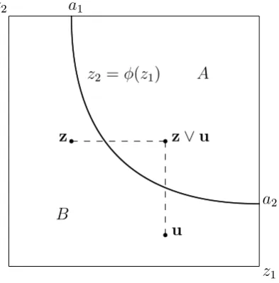
Figure 1 below illustrates the optimal stopping rule. A is the set of (z1; z2) which
satis…es (2) and let us refer to it as the acceptance set. Then when there are no price di¤erences across …rms, a consumer will stop searching if and only if the maximum utility pair so far lies within A. Let B be the complement of A.
z1
z2
A
B a1
a2
zr r
r
z_u
u z2 = (z1)
Figure 1: The optimal stopping rule in multiproduct search
De…ne the border ofA asz2 = (z1)(i.e.,(z1; (z1))satis…es (2) with equality) and call
it thereservation frontier. The reservation frontier is decreasing and convex. From the de…nition of ( ), one can check that
0(z
1) =
1 F1(z1)
1 F2( (z1))
<0 ;
and so ( ) is a decreasing function. Then it is also easy to see that 0(z1) increases
with z1, i.e., ( ) is convex.15
15If we consider two intrinsic complements, the reservation frontier may no longer be decreasing.
For example, when the utility function takes the form ofu1+u2+ u1u2 with >0, one can check
that in the duopoly case, for instance, the reservation frontier satis…es
1
2(1 u1) 2+1
2(1 u2) 2+
4 (u1 u2)
2+ (1 u
1u2)2 =s ;
Notice that ai on Figure 1 is just the reservation utility level when the consumer is only searching for producti. (If all productihave the same price, a consumer will stop searching if and only if the maximum utility so far is no less than ai.) It solves
i(ai) = s ; (3)
and satis…es (a1) = u2 and (u1) = a2. This is because when the maximum possible
utility of one product has been achieved, the consumer will behave as if she is only searching for the other product.
Search behavior comparison. It is useful to compare consumer search behavior be-tween single-product and multiproduct search. The early literature has emphasized that in both cases (given additive utilities in the multiproduct case) the optimal stop-ping rule possesses the static reservation property. Despite this similarity, consumers’ search behavior exhibits some important di¤erences between the two cases, which have not been discussed before.
In single-product search with perfect recall, the stopping rule is characterized by a reservation utility a. When a consumer is already at some …rm (except the last one), she will stop searching if and only if the current product has a utility greater than
a. Previous o¤ers are irrelevant because they must be worse than a (otherwise the consumer would not have come to this …rm). As a result, a consumer never returns to previously visited …rms until she …nishes sampling all …rms. In particular, if there are an in…nite number of …rms, the consumer never exercises the recall option.
However, in multiproduct search, a consumer’s stopping rule depends on both the current …rm’s o¤er u and the best o¤er so far z. This can be seen from the example
indicated in Figure 1, where the current o¤er u lies outside the acceptance set A but
the consumer will stop searching because z_u 2 A (where _ denotes the “join” of
two vectors). When she stops searching, she will go back to some previous …rm to buy product 2. This has two implications for the demand analysis. First, with multiproduct search, a …rm’s price adjustment will not only a¤ect a consumer’s search decision at this …rm, but will also a¤ect her search decisions at subsequent …rms if she leaves this …rm. Second, a consumer often returns to a previously visited …rm to buy one product even if there are …rms left unsampled. This is true even if there are an in…nite number of …rms.
These di¤erences will complicate the demand analysis in multiproduct search. More-over, unlike the single-product search case, considering an in…nite number of …rms does not achieve any simplicity. In e¤ect, with multiproduct search, the simplest case is when there are only two …rms. Hence, in the following analysis, I mainly deal with the duopoly case. As I will discuss in section 5.1, such a simpli…cation does not lose the most important insights concerning …rm pricing in a multiproduct search market. (A detailed analysis of the general case with more than two …rms is provided in the online
supplementary document at https://sites.google.com/site/jidongzhou77/research.)
3
Equilibrium Prices
3.1
The single-product benchmark
To facilitate comparison, I …rst report some results from the single-product search model (see Wolinsky, 1986 and Anderson and Renault, 1999 for an analysis with n
…rms). Suppose the product in question is product i, and the unit search cost is still
s. Then the reservation utility level is ai de…ned in (3), and it decreases with s (i.e., a higher search cost will make consumers less willing to search on). In the following analysis, I mainly focus on the case with a relatively small search cost:
s < i(ui),ai > ui for bothi= 1;2: (4)
(Remember that i(ui) is the expected bene…t from sampling another product i when the current one has the lowest possible match utility.) This condition ensures an active search market even in the single-product case.
The symmetric equilibrium price p0
i in the duopoly case is then determined by
1 p0 i
=fi(ai)[1 Fi(ai)] + 2
Z ai
ui
fi(u)2du
| {z }
0
: (5)
It follows thatp0
i increases with the search cost s (or decreases with ai) if
fi(ai)2 +fi0(ai)[1 Fi(ai)] 0:
This condition is equivalent to an increasing hazard ratefi=(1 Fi). Then we have the following result (Anderson and Renault, 1999 have shown this result for an arbitrary number of …rms):
Proposition 1 Suppose the consumer is only searching for product i and the search cost condition (4) holds. Then the equilibrium price de…ned in (5) increases with search costs if the match utility has an increasing hazard rate fi=(1 Fi).
3.2
Equilibrium prices in multiproduct search
I now turn to the multiproduct search case. Let(p1; p2) be the symmetric equilibrium
prices. For notational convenience, let(u1; u2) be the match utilities of …rm I, the …rm
in question, and(v1; v2)be the match utilities of …rm II, the rival …rm. In the symmetric
equilibrium, for a consumer who samples …rm I …rst, her reservation frontieru2 = (u1)
is determined by
which simply says that the expected bene…t of sampling …rm II is equal to the search cost. Note that (u1) is only de…ned for u1 2 [a1; u1] (see Figure 2 below). But
for convenience, let us extend its domain to all possible values of u1, and stipulate
(u1)> u2 foru1 < a1.
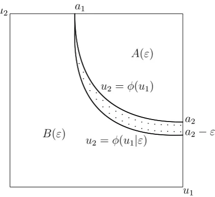
Instead of writing down the demand functions and deriving the …rst-order conditions for the equilibrium prices directly, I use the following economically more illuminating method. Starting from an equilibrium, suppose …rm I unilaterally decreases p2 by a
small". How does this adjustment a¤ect …rm I’s pro…ts? Let us focus on the …rst-order e¤ects. First, …rm I su¤ers a loss from those consumers who only buy product 2 from it because they are now paying less. Since in equilibrium half of the consumers buy product 2 from …rm I (remember the assumption of full market coverage), this loss is
"=2. Second, …rm I gains from boosted demand: (i) For those consumers who visit …rm I …rst, they will be more likely to stop searching since they hold equilibrium beliefs that the second …rm is charging the equilibrium prices. Once they stop searching, they will buy both products from …rm I immediately. (ii) For those consumers who eventually sample both …rms, they will be more likely to buy product 2 from …rm I due to the price reduction. In equilibrium, the loss and gain should be such that …rm I has no incentive to deviate, which generates the …rst-order condition forp2.
Now let us analyze in detail the two (…rst-order) gains from the proposed small price reduction. The …rst gain is from the e¤ect of the price reduction on consumers’ search decisions. How many consumers who sample …rm I …rst will stop searching because of the price reduction? (Note that the consumers who sample …rm II …rst hold equilibrium beliefs and so their stopping decisions remain unchanged.)
Denote by (u1j") the new reservation frontier. Since reducingp2 by"is equivalent
to increasingu2 by ", (u1j") solves
1(u1) + 2( (u1j") +") =s ;
so (u1j") = (u1) " according to the de…nition of ( ). That is, the reservation
frontier moves downward everywhere by ", and the stopping region A expands (i.e., more consumers buy immediately at …rm I) as illustrated in Figure 2 below.16 For a
small ", the number of consumers who originally continued to search but now cease searching and buy immediately at …rm I (i.e., the probability measure of the shaded area between (u1) and (u1j") in Figure 2) is
" 2
Z u1
a1
f(u; (u))du : (7)
(Remember that half of the consumers sample …rm I …rst. The integral term is the line integral along the reservation frontier in theu1 dimension.)
16More precisely, (a
1j") = u2 " and so the reservation frontier has a small vertical segment at
u1
u2
A(")
B(")
u2 = (u1)
u2 = (u1j")
a1
a2 "
a2
[image:14.595.199.419.79.280.2]p p p p p p p p p p p p p p p p p p p p p p p p p p p p p p p p p
Figure 2: Price deviation and the stopping rule
What is …rm I’s net bene…t from these marginal consumers? Realize that these marginal consumers now buy both products from …rm I for sure, while before the price deviation they only bought each product from …rm I with some probability less than one (i.e., when they search on but …nd worse products at …rm II). To be speci…c, consider a marginal consumer on the reservation frontier with match utilities (u1; (u1)). If she
chooses to sample …rm II, she will …nd a worse product 1 at …rm II (i.e., v1 < u1)
with probability F1(u1), in which case she will return to …rm I and buy its product 1.
Similarly, if she continues to sample …rm II, she will …nd a worse product 2 at …rm II (i.e., v2 < (u1)) with probabilityF2( (u1)), in which case she will return to …rm I
and buy its product 2. Hence, the net bene…t from inducing this marginal consumer to cease searching is p1[1 F1(u1)] +p2[1 F2( (u1))]. We then sum this bene…t over all
marginal consumers on the reservation frontier. By using (7), this total bene…t is
" 2
Z u1
a1
fp1[1 F1(u)] +p2[1 F2( (u))]gf(u; (u))du : (8)
The second gain is from those consumers who sample both …rms. They will now more likely buy product 2 from …rm I due to the price reduction. Consider …rst a consumer who visits …rm I …rst and …nds match utilities (u1; u2) 2 B("). She will
then continue to visit …rm II, but will return to …rm I and buy its product 2 if v2 <
u2 +". The probability of that event is F2(u2 +") F2(u2) +"f2(u2). So the small
price adjustment increases the probability that this consumer buys product 2 from …rm I by "f2(u2). Then the total increased probability from all such consumers is
" 2
R
B(")f2(u2)dF(u) " 2
R
at …rm I is "2RBf2(v2)dF(v). Adding them together gives us the second gain, which is
p2"
Z
B
f2(u2)dF(u) : (9)
In equilibrium, the (…rst-order) loss "=2 from the small price reduction should be equal to the sum of the two (…rst-order) gains in (8) and (9). This yields the …rst-order condition for p2:
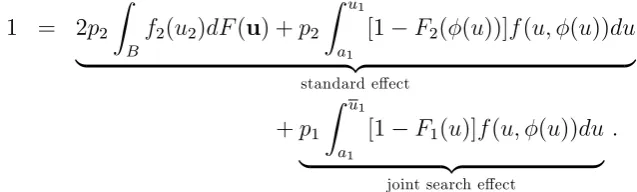
1 = 2p2
Z
B
f2(u2)dF(u) +p2
Z u1
a1
[1 F2( (u))]f(u; (u))du
| {z }
standard e¤ect
(10)
+p1
Z u1
a1
[1 F1(u)]f(u; (u))du
| {z }
joint search e¤ect
:
The …rst two terms on the right-hand side capture the standard e¤ect of a product’s price adjustment on its own demand: reducingp2 increases demand for product 2. (This
is similar to the right-hand side of (5) in the single-product search case.)
The last term, however, captures a new feature of the multiproduct search model: when …rm I reduces its p2, more consumers who sample it …rst will stop searching and
buy both products, which increases the demand for its product 1 as well. This makes the two products supplied by the same …rm like complements even if they are physically independent.17 This e¤ect occurs because each consumer is searching for two products
and the cost of search is incurred jointly for them, and so I refer to it as thejoint search e¤ect henceforth.
[image:15.595.137.456.193.289.2]Also notice that the size of the joint search e¤ect (which determines the degree of “complementarity” between the two products in each …rm) relies on the mass of marginal consumers on the reservation frontier, i.e., (7). It depends not only on the density function f but also on the “length” of the reservation frontier as indicated in Figure 2. For example, in the uniform distribution case, when the search cost increases, the reservation frontier becomes longer such that the mass of marginal consumers rises and thus the two products in each …rm become more like complements. As we shall see below, this observation plays an important role in …rms’ pricing decisions.
Similarly, one can derive the …rst-order condition forp1:
1 = 2p1
Z
B
f1(u1)dF(u) +p1
Z u2
a2
[1 F1( 1(u))]f( 1(u); u)du (11)
+p2
Z u2
a2
[1 F2(u)]f( 1(u); u)du ;
17Notice that the complementarity caused by the joint search cost is di¤erent from intrinsic
where 1 is the inverse function of . The …rst two terms on the right-hand side re‡ect the standard e¤ect of adjusting price p1, and the last term captures the joint search
e¤ect. I summarize the results in the following lemma:18
Lemma 2 Under the search cost condition (4), the …rst-order conditions for p1 andp2
to be the equilibrium prices are given in (10) and (11).
Both (10) and (11) are linear equations in prices, and the system of the two prices has a unique solution. Thus, the symmetric equilibrium, if it is characterized by the …rst-order conditions, will be unique. Notice that if …rms ignored the joint search e¤ect, then the pricing problem would be separable between the two products. A special case is when s = 0 (so ai = ui and B equals the whole match utility domain). Then the e¤ect of a price adjustment on consumer search behavior (i.e., (8)) disappears, and the …rst-order conditions simplify to
1 pi
= 2
Z ui
ui
fi(u)2du : (12)
In this case, the multiproduct model yields the same equilibrium prices as the single-product model.
In the following analysis, I will often rely on the case with two symmetric products. Slightly abusing the notation, let the one-variable functions F( ) and f( ) denote the common marginal distribution function and density function, respectively. Leta be the common reservation utility in each dimension. In particular, with symmetric products, we havef(u1; u2) =f(u2; u1) and the reservation frontier satis…es ( ) = 1( ), i.e., it
is symmetric around the 45-degree line in the match utility space. Ifpis the equilibrium price of each product, then both (10) and (11) simplify to
1
p = 2
Z
B
f(ui)f(ui; uj)du+
Z u
a
[1 F( (u))]f(u; (u))du
| {z }
standard e¤ect:
(13)
+
Z u
a
[1 F(u)]f(u; (u))du
| {z }
joint search e¤ect:
:
18One can also derive the …rst-order conditions by calculating the demand functions directly. For
example, when …rm I unilaterally deviates to(p1 "1; p2 "2), the demand for its product 1 is
1 2
Z u1
u1
[1 H2( (u1j")ju1)(1 F1(u1+"1))]dF1(u1) +1
2
Z u1
u1
H2( (v1)jv1)(1 F1(v1 "1))dF1(v1);
where"= ("1; "2), (u1j") = (u1+"1) "2 is the reservation frontier associated with the deviation,
and Hi(j) is the conditional distribution function. Consumers who sample …rm I …rst will buy its
Discussion: the second-order conditions and asymmetric equilibria. In our multi-product search model, it is di¢cult to investigate the second-order conditions in general. In the online supplementary document, I show that in the case of symmetric products and independent match utilities, each …rm’s pro…t function is locally concave around the price de…ned in (13) under fairly general conditions. In the examples with uniform and exponential distribution (which are used for illustration below), it can be numerically veri…ed that a …rm’s pro…t function is globally quasi-concave, and thus the …rst-order conditions are su¢cient for the equilibrium prices.
A related issue is the possible existence of a type of asymmetric equilibrium where …rms put di¤erent products on sale. For example, in the case with symmetric products, one …rm may charge price pL for its product 1 and price pH > pL for its product 2, and the other …rm sets prices in the opposite way. However, as shown in the online supplementary document, this type of equilibrium cannot be sustained at least when the two symmetric products have independent match utilities andf is logconcave.
For illustration of the equilibrium prices, I present two examples:
The uniform example: Suppose u1 and u2 are independent, and ui s U[0;1]. Then
i(x) = (1 x)2=2. So a = 1 p
2s, and condition (4) requires s 1=2. The reservation frontier satis…es
(1 u)2+ (1 (u))2 = 2s ;
so the stopping regionA is a quarter-disk with radius p2s. Then (13) implies
p= 1
2 (12 1)s ; (14)
where 3:14is the mathematical constant. (The standard e¤ect is = 2 s =2, and the joint search e¤ect is =s.)19
The exponential example: Suppose u1 and u2 are independent, and fi(ui) = e ui for
ui 2 [0;1). Then i(x) = e x. So e a = s, and the search cost condition (4) requires s 1. The reservation frontier satis…es
e u +e (u) =s ;
so (u) is one branch of a hyperbola. Then (13) implies
p= 1
1 + 1 6s3
:
(The standard e¤ect is = 1, and the joint search e¤ect is =s3=6.)
The price increases with search costs in the uniform example, but it decreases with search costs in the exponential example. As I will explain below, the result that prices can decline with search costs is not exceptional in the multiproduct search model.
19The …rst term in (13) is2R
Bdu, so it equals two times the area of regionB, i.e.,2(1 s =2) = 2 s .
The second term in (13) isRa1[1 (u)]du, which is the area of regionAand so equalss =2. The joint
3.3
Price and search cost
This section investigates how prices vary with search costs. When search costs rise, there are two e¤ects: First, consumers will become more reluctant to shop around, and so fewer of them will sample both …rms (i.e., the region of B shrinks). This always induces …rms to raise their prices. Second, when search costs rise, the mass of mar-ginal consumers on the reservation frontier also changes. If the number of marmar-ginal consumers increases with search costs (which is true, for instance, in the uniform dis-tribution case where the reservation frontier becomes “longer” as search costs rise in the permitted range of (4)), …rms have an incentive to reduce prices. This incentive is further strengthened in the multiproduct case due to the joint search e¤ect: stopping a marginal consumer from continuing to search can boost demand for both products. The …nal prediction depends on which e¤ect dominates.
I introduce the following regularity condition:
hi(uijuj)
1 Fi(ui)
increases with ui for any givenuj . (15)
In particular, if the two products have independent match utilities, this condition is just the standard regularity condition of increasing hazard rate in the single-product case.
In the following, I focus on the case with two symmetric products, and so the equilibrium price p is given in (13).20 One can see that p increases with search costs if
and only if @@s+@@s <0, where is the standard e¤ect and is the joint search e¤ect as de…ned in (13). As the following proposition indicates, @@s <0if the regularity condition (15) holds. This means that if the joint search e¤ect were absent, prices would increase with search costs under the condition (15), similar as in the single-product scenario.
However, taking into account the joint search e¤ect can qualitatively change the picture. As indicated in the following proposition, the joint search e¤ect can vary with s in either direction. If @@s <0, the joint search e¤ect will reinforce the standard e¤ect such that the price increases with search costs even faster. Conversely, if @@s >0
(e.g., when the conditional density is weakly decreasing), the joint search e¤ect will mitigate or even overturn the usual relationship between price and search costs. As a result, the regularity condition (15) is not enough to ensure that prices increase with search costs in our model. The following result gives a new condition (all omitted proofs can be found in Appendix A):
20Product asymmetry is another force that could in‡uence the relationship between prices and search
costs. Intuitively, when one product has a lower pro…t margin than the other, the joint search e¤ect from adjusting its price is stronger (i.e., reducing its price can induce consumers to buy the other more pro…table product). Then this product’s price may go down with the search cost. For example,
when product 1 has a match utility uniformly distributed on[0;1]and product 2 has a match utility
Proposition 2 Suppose the search cost condition (4) holds, and the two products are symmetric. Then p de…ned in (13) increases with search costs if and only if
Z u
a
f( (u))
1 F( (u))ff(u)h(uj (u)) + [1 F(u)]h
0(uj (u))gdu
| {z }
@ @s
> f(a; u)
Z u
a
h0(uj (u))f( (u))du
| {z }
@ @s
:
(16)
If the two products further have independent match utilities, a su¢cient condition for (16) is that the marginal density f(u) is (weakly) increasing.
The condition (16), however, can be easily violated (such that prices decrease with search costs) even under the regularity condition of (15).21 For example, in the
ex-ponential example with independent match utilities, @
@s = 0 and @
@s > 0, and so the opposite of (16) holds. Other simple examples include the distribution with decreasing density f(u) = 2(1 u) and the logistic distribution f(u) = eu=(1 +eu)2 when search
costs are relatively small. As we have argued, this surprising result is due to the joint search e¤ect, the new economic force in our multiproduct search model.
If …rms supply (and consumers need) more products, the joint search e¤ect could have an even more pronounced impact such that prices fall with search costs more likely. In Appendix A, I extend the two-product model to the case with m products. In particular, in the uniform case with m symmetric products, the equilibrium price p
has a simple expression:
1 p = 2
Vm( p
2s) 2m
| {z }
standard e¤ect
+(m 1)Vm(
p
2s) 2m 1
| {z }
joint search e¤ect
; (17)
wheres2[0;1=2]and Vm(r)is the volume of an m-dimensional sphere with radiusr.22 One can check thatpincreases withsif and only ifm <1+ =2 2:6. Therefore, when consumers search for more than two products, even in the uniform example, prices start to decrease with search costs.
Discussion: large search costs. Our analysis so far has been restricted to relatively small search costs such that it is even worthwhile to search for one good alone. I now discuss the case with larger search costs beyond condition (4). (In some circumstances,
21If the opposite of (15) holds, the left-hand side of (16) is negative, and meanwhile h0 must be
negative such that the right-hand side is positive. Thus, (16) will fail to hold and so the pricepwill
decrease with search costs. This is not surprising, because even in the single-product search case (5) implies that the equilibrium price decreases with search costs if the match utility has a decreasing hazard rate. What is more surprising in the multiproduct search model is that prices can decrease with search costs even under the regularity condition.
22The volume of an m-dimensional sphere with radius r is V
m(r) = (r
p )m
(1+m=2), where ( ) is the
Gamma function. One can show that for any …xedr,limm!1Vm(r) = 0. Then asmgoes to in…nity,
pwill approach the perfect information price1=2in expression (12). This is because for a …xed search
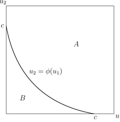
a consumer conducts multiproduct search because it is not worthwhile to search for each good separately.) As we shall see later, this discussion will also be useful for understanding the results in the bundling case. For simplicity, let us focus on the case of symmetric products. Suppose the condition (4) is violated such that s > i(u) and
a < u. (But s cannot exceed 2 i(u) to ensure an active search market.) Then the reservation frontier is shown in Figure 3 below, wherec= (u).
u1
u2
A
B c
[image:20.595.199.396.196.396.2]c u2 = (u1)
Figure 3: The optimal stopping rule with large search costs
The key di¤erence between this case and the case of small search costs is that now the reservation frontier becomes “shorter” as search costs go up. This feature has a signi…cant impact on how prices vary with search costs. For example, in the uniform case, a higher search cost now leads to fewer marginal consumers on the reservation frontier, which provides …rms with a greater incentive to raise prices. (In this case, the joint search e¤ect strengthens the usual relationship between prices and search costs.) I show in the online supplementary document that if the two products are symmetric and they have independent match utilities, and if search costs are relatively high such that i(u)< s <2 i(u), then the equilibrium pricepincreases with search costs if each product’s match utility has a monotonic density and a (weakly) increasing hazard rate.
3.4
Price comparison with single-product search
As the end of this section, I compare the multiproduct search prices in section 3.2 with the single-product search prices in section 3.1, and discuss one empirical implication of the comparison result.
Proposition 3 Suppose the search cost condition (4) and the regularity condition (15) hold. Then pi p0i; i = 1;2; i.e., each product’s price is lower in multiproduct search
This result is intuitive. In our model, there are economies of scale in search (i.e., searching for two products is as costly as searching for only one), so more consumers are willing to sample both …rms in multiproduct search, which intensi…es the price competition. On top of that, the joint search e¤ect gives rise to a complementary pricing problem and induces …rms to further lower their prices. For example, in the uniform case with s= 0:1, the multiproduct search price in (14) is0:51, lower than the single-product search price 0:64by 20%. (Notice that p0 = 1=(2 p2s) in the
single-product case.) It is worth emphasizing that even if economies of scale in search are weak (e.g., when single-product search is less costly than multiproduct search), the joint search e¤ect can still induce substantial price reduction. For instance, in the uniform case, if product search is half as costly as two-product search (i.e., if the single-product search cost is s=2), then the single-product search price becomes 1=(2 ps). The multiproduct search price is still signi…cantly lower than that. For example, when
s= 0:1, the new single-product search price is 0:59, and the multiproduct search price
0:51 is still lower than it by13:5%.
As documented in Warner and Barsky (1995), MacDonald (2000), Chevalier, Kashyap, and Rossi (2003) and others, prices of many retail products fall during demand peaks such as holidays and weekends. (All these paper use data from multiproduct retailers such as supermarkets and department stores.) This phenomenon is termed counter-cyclical pricing. A simple extension of the multiproduct search model can provide a possible explanation for this phenomenon.23 Suppose there are now both single-product
and multiproduct searchers in the market. Suppose a higher proportion of consumers become multiproduct searchers during high-demand periods such as weekends and hol-idays. (For example, many households conduct their weekly grocery shopping during weekends, and more people buy multiple gifts in Christmas season.24) Then Proposition
3 immediately implies that market prices will decline.
For illustration, I consider an example where there are two symmetric products and each product is needed by a consumer with a probability 2 [0;1]. (Our basic model corresponds to = 1.) Suppose the need for each product occurs independently across products and consumers. Then there are three groups of consumers in the market: a fraction of 2 of consumers are searching for both products, a fraction of 2 (1 )
of consumers are searching for only one product, and the rest need none of them. A demand rise can be re‡ected by an increase of .
23There are of course other possible explanations for countercyclical pricing. For example, it may
be due to the dynamic interaction among competing retailers, who are more likely to have a price war during demand booms (Rotemberg and Saloner, 1986). It may also be because retailers advertise price information more intensely during high-demand periods, or because more low-income consumers who are usually more price sensitive enter the market.
24Another possible justi…cation is that the demand ‡uctuations may also arise endogenously:
The equilibrium price for each product in this extended model is given by
1
p = (1 ) 0+ ( + ) ;
where 0 is the right-hand side of (5), and and are the standard e¤ect and the joint
search e¤ect in multiproduct search, respectively. (Conditional on a consumer buying one product, this consumer is a single-product searcher with probability 1 and a multiproduct searcher with probability .) Proposition 3 implies that 0 < + , so
p decreases with . This result is due to both 0 < (which re‡ects the economies of
scale in search) and >0 (which re‡ects the joint search e¤ect).
Warner and Barsky (1995) have suggested an explanation based on consumer search for countercyclical pricing, though they did not develop a formal search model. Their idea is wholly based on economies of scale in search, while my model suggests that even if economies of scale in search are weak, the joint search e¤ect can still induce multiproduct …rms to reduce their prices substantially. In e¤ect, one argument in Chevalier, Kashyap, and Rossi (2003) against Warner and Barsky’s explanation is that they did not …nd clear evidence that consumers become signi…cantly more price elastic during peak-demand periods. However, they only consider each product (category)’s own-price elasticity. According to our model, the cross-price elasticity due to the joint search e¤ect may play an important role in multiproduct retailers’ pricing decisions. Taking that into account may enhance the explanatory power of a search model for countercyclical pricing.
4
Bundling in Search Markets
Bundling is a widely used multiproduct pricing strategy. One adopted form, termed
pure bundling, is that the …rm sells several products in a package (e.g., software suites, TV program packages, and music albums), and none of them is available for individual purchase. The other form, termed mixed bundling, is that alongside each separately available product, a package is sold at a discount relative to the components. For ex-ample, retailers such as electronic stores, travel agencies and online book shops often o¤er a customer a discount if she buys more than one product from the same store. An-other related example in the retail market is that the shipping fee is often independent of the number of products (e.g., furniture items) in the same order.
To illustrate the main insights in a simple way, I focus on the case of pure bundling. (The case of mixed bundling is more complicated to analyze, but the main results derived in the pure bundling case hold qualitatively there. See the online supplementary document for the details.) I assume that when …rms bundle, consumers buy only one of the two bundles, i.e., they will not buy both bundles to mix and match. This is the case, for instance, when pure bundling introduces the compatibility problem, or when the bundle price is so high that it is not worthwhile to buy both bundles.25
Bundling and search incentive. I …rst examine how bundling might a¤ect con-sumers’ search incentive. In the linear pricing case, given match utilities(u1; u2)at …rm
I, the expected bene…t from sampling …rm II is
E max 0;P2i=1(vi ui); v1 u1; v2 u2 : (18)
(This merely rewrites the left-hand side of (6). The expectation operator is over(v1; v2).)
If both products at …rm II are a worse match, the consumer will return and buy at …rm I and so the gain from the extra search will be zero; if both products at …rm II are a better match, the consumer will buy at …rm II and gainP2i=1(vi ui); if only product
i at …rm II is the better match, she will mix and match and the gain will bevi ui. Suppose now both …rms adopt the pure bundling strategy and charge the same prices. Then the expected bene…t from sampling …rm II becomes
E[ max(0;P2i=1(vi ui))]; (19)
since the opportunity to mix and match has been completely ruled out. This bene…t is clearly smaller than (18). Therefore, compared to linear pricing, bundling reduces consumers’ search incentive and induces them to stop at the …rst sampled …rm more often.26
When both …rms bundle, consumers in e¤ect face a single-product search problem: …rm I o¤ers a composite product with a match utility U =u1+u2, and …rm II o¤ers
another one with an independent match utility V = v1 +v2. Both U and V belong
to [U = u1+u2; U = u1 +u2]. Let G( ) and g( ) denote their common cdf and pdf,
respectively. Denote bybthe reservation utility level in this search problem. It satis…es
Z U
b
(U b)dG(U) = s : (20)
The left-hand side is the expected bene…t from sampling the second bundle given the …rst one has a match utilityb. Hence, in a symmetric equilibrium a consumer will visit
25For example, in the uniform example below, when the search cost is relatively high, the bundle
price is greater than1. Then even if …rm I’s products have match utilities(1;0)and …rm II’s products
have match utilities(0;1), it is not worthwhile to buy both bundles.
26In the case of mixed bundling, the joint-purchase discount, which is the di¤erence between the
the second …rm if and only if the …rst bundle has a match utilityu1+u2 belowb. Since
pure bundling reduces consumers’ search incentive, the acceptance set expands, i.e.,
[image:24.595.200.399.189.389.2]b < u1+ (u1) for any u1 2[a1; u1].
Figure 4 below illustrates this change of the consumer stopping rule, where the linear line is the reservation frontier in the pure bundling case and the new acceptance set is
A plus the shaded area.
u1
u2
A
u2 = (u1)
u2 =b u1
a1 a2 @ @ @ @ @ @ @ @ @ @ @ @ @ @ @@ p p p p p p p p p p p p p p p p p p p p p p p p p p p p p p p p p p p p p p p p p p p p p p p p p p p p p p p p p p p p p p p p p p p p p p p p p p p p p p p p p p p p p p p p p p p p p p p p p p p p p p p p p p p p p p p p p p p p p p p p p p p p p p p p p p p p p p p p p p p p p p p p p p p p p p p p p p p p p p p p p p p p p p p p p p p p p p p p p p p p p p p p p p p p p p p p p p p p
Figure 4: The optimal stopping rule: linear pricingvs pure bundling
As I will demonstrate below, this search-discouraging e¤ect of bundling may make …rms compete less aggressively and reverse the usual welfare impact of competitive bundling.
Incentive to bundle. Starting from the linear pricing equilibrium, does a …rm have a unilateral incentive to introduce bundling in a search environment? Suppose that …rms choose prices and whether to bundle products simultaneously,27 and both
choices are unobservable to consumers until they reach the store.
When a …rm unilaterally introduces pure bundling, it will make more consumers who visit it …rst stop searching and buy immediately. (For these consumers, the situation is now actually equivalent to both …rms adopting the bundling strategy.) But bundling will also exclude some consumers who continue to search and would otherwise come back and buy a single product. The following result shows that with costly search, the …rst positive e¤ect always dominates.
Proposition 4 In the duopoly model with costly search (s >0), starting from the linear pricing equilibrium, each …rm has a unilateral incentive to introduce the pure bundling strategy.
Proof. Each …rm earns (p1+p2)=2 in the linear pricing equilibrium. Now consider
the following deviation: …rm I unilaterally bundles its products and sells the bundle at
a price p1 +p2. (Before they reach …rm I, consumers still hold the equilibrium belief
that …rm I is setting linear prices.) Since this deviation does not change the bundle price, it su¢ces to show that more than half of the consumers will buy the bundle from …rm I after the deviation. Notice that if both …rms bundle and charge the same price, each will have demand 1=2. So it su¢ces to show that more consumers will buy the bundle from …rm I in the deviation case than in the pure bundling case with the bundle price p1+p2.
Consider …rm I’s two demand sources: (a) For those consumers who sample …rm I …rst, they will act as in the pure bundling case. So the demand from them is the same as in the pure bundling case. (b) For those consumers who sample …rm II …rst, they will adopt the stopping rule in the linear pricing case. So compared to the pure bundling case, more consumers (i.e., those on the shaded area in Figure 4) will come to …rm I. (This argument relies on costly search. If the search cost is zero, all consumers who sample …rm II …rst will come to …rm I in either case.) But once they arrive at …rm I and …nd out its bundling strategy, they will make choices as in the pure bundling case. Hence, in the deviation case, the demand from those consumers who sample …rm II …rst is greater than in the pure bundling case. Combining (a) and (b) proves the result.
It is also easy to see that starting from the situation where both …rms bundle (and consumers believe so), no …rm has a unilateral incentive to unbundle. This is simply because given consumers’ beliefs and the rival’s bundling strategy, unilaterally unbundling has no impact at all on the market. Therefore, if …rms choose prices and their bundling strategies simultaneously, the only symmetric equilibrium is a bundling equilibrium.
Comparison with linear pricing. When …rms bundle, we have in e¤ect a single-product search problem. Let P be the symmetric equilibrium bundle price. Then, similar to (5),P is determined in
1
P =g(b)[1 G(b)] + 2
Z b
U
g(U)2dU ; (21)
where the reservation utility b has been de…ned in (20). P increases with search costs provided that U = u1 +u2 has an increasing hazard rate (which is true, for example,
when each ui has an increasing hazard rate and is independent from uj, as shown by Miravete, 2002).
When information is perfect, Matutes and Regibeau (1988), Economides (1989), and Nalebu¤ (2000) have shown in a two-dimensional Hotelling setting (with unit demand and full market coverage) that pure bundling typically lowers price (and pro…t) and boosts consumer welfare. This is mainly because pure bundling makes a price reduction doubly pro…table, thereby intensifying price competition, and the price reduction is large enough to outweigh the restriction of choices available with pure bundling.
a=uand b=U) pure bundling results in a lower bundle price (P <2p) if and only if
Z u
u
f(u)2du <2
Z U
U
g(U)2dU : (22)
With independent match utilities, one can check that this condition holds for a large range of distributions such as uniform, normal and logistic. But it does not always hold. For instance, as we will see below, in the exponential case the equality of (22) holds. (However, as implied by Proposition 5 below, if consumers buy a large number of products, pure bundling always leads to a lower bundle price than linear pricing in the perfect information case.)
When search is costly, the pro-competitive e¤ect of pure bundling still applies to those consumers who sample both …rms. However, pure bundling weakens consumers’ search incentive and so reduces the number of informed consumers in the …rst place, which tends to soften price competition. The net e¤ect hinges on the relative importance of these two forces. Intuitively, when the search cost is higher, there will be fewer fully informed consumers, and then the …rst e¤ect will be less important and pure bundling may lead to a higher bundle price. This intuition is con…rmed in our two examples:
The uniform example: Suppose u1 and u2 are independent, and ui s U[0;1]. To facilitate the comparison with linear pricing, we keep the search cost condition
s 1=2. One can show that G(U) = U2=2 and g(U) = U if U 2 [0;1], and
G(U) = 1 (2 U)2=2 and g(U) = 2 U if U 2 [1;2]. According to (20), the
reservation utilityb satis…es (2 b)3=6 = s if s 2[0;1=6] (so b 1 in this case),
and 1 b+b3=6 =s if s2[1=6;1=2] (sob <1 in this case). Then (21) implies
P =
8 > > > > <
> > > > :
1
4 3 s
if s2[0;1 6)
1
1 6b3+b
if s2[16;12] :
One can check thatP increases withs, but the speed is much faster whens 1=6. (The upward sloping curve in Figure 5(a) below depicts how P 2p varies with search costs.) This is because in the range of s 2 [0;1=6), b > 1 and so as
s increases, the reservation frontier gets “longer” (i.e., there are more marginal consumers on the frontier), which mitigates …rms’ incentive to raise prices. By contrast, afters exceeds 1=6, b <1 and so the reservation frontier gets “shorter” ass increases, which strengthens …rms’ incentive to raise prices. In other words, when the reservation frontier is still getting longer in the linear pricing case, it already starts to get shorter in the bundling case. In particular, when the search cost exceeds about0:26, the bundle price is higher in the pure bundling case than in the linear pricing case.
The exponential example: Suppose u1 and u2 are independent, and fi(ui) = e ui for
strictly increasing hazard rate, thoughui has a constant one.) According to (20), the reservation utility b satis…es (2 +b)e b = s. Substituting G and g into (21) yields
P = 2
1 e 2b ;
which increases withs and is always greater than the bundle price2pin the linear pricing case (except P = 2p at s = 0). (The upper curve in Figure 5(b) depicts how P 2p varies with search costs in this example.) With pure bundling, as s
increases the reservation frontier always gets “shorter” in the exponential case, which explains why pure bundling reverses the relationship between price and search costs.
Now let us examine the welfare impact of pure bundling relative to linear pricing. The …rst observation is that total welfare—de…ned as the sum of industry pro…t and consumer surplus—must fall with bundling. With the assumption of full market cover-age, consumer payment is a pure transfer and so only the match e¢ciency (including search costs) matters. Bundling reduces e¢ciency because it not only results in insu¢-cient consumer search (i.e., too few consumers search beyond the …rst sampled …rm due to bundling) but also rules out the opportunity to mix and match for the consumers who sample both …rms. This general result holds no matter whether information frictions exist or not.
0.1 0.2 0.3 0.4 0.5
-0.6 -0.4 -0.2 0.0 0.2 0.4 0.6
s
profit
consumer surplus
(a): uniform example
0.1 0.2 0.3 0.4 0.5 0.6 0.7 0.8 0.9 1.0
-0.4 -0.2 0.0 0.2 0.4
s
profit
consumer surplus
[image:27.595.95.501.432.593.2](b): exponential example
Figure 5: The welfare impact of pure bundling
relative to linear pricing, pure bundling bene…ts consumers when search costs are lower than about 0:24, but it harms consumers when search costs exceed that threshold. In the exponential case, pure bundling always harms consumers since it (weakly) raises the bundle price for any search cost level. This is indicated by the lower curve in Figure 5(b). (Calculating consumer surplus directly in our multiproduct search framework is complicated. In Appendix B, I develop a more e¢cient indirect method.)
In sum, in a search environment pure bundling can generate a signi…cant competition-relaxing e¤ect such that relative to linear pricing it can bene…t …rms and harm con-sumers, in contrast to the perfect information case.28
Nevertheless, this search-based e¤ect is most pronounced when the number of goods a consumer is looking for is relatively small. If a consumer is looking for a large number of goods and if the search cost is …xed, she will almost surely sample both …rms, and the situation will be close to the perfect information case. Then, as the following result shows, the pro-competitive e¤ect of pure bundling will dominate.
Proposition 5 For given search costs, if each …rm supplies (and each consumer needs) a large number of symmetric products with independent match utilities, then compared to linear pricing, pure bundling leads to a lower bundle price and so lower industry pro…ts, and it bene…ts consumers iff is logconcave.
This result is not trivial, and it has not been noticed in the existing literature. Pure bundling leads to lower prices, but it also lowers match e¢ciency. What I show in the proof is that the bundle price increases with the number of products much slower in the pure bundling case than in the linear pricing case, such that the price e¤ect eventually dominates the match e¤ect and consumers become better o¤.
5
Concluding Discussion
This paper has two contributions: First, it developed a tractable multiproduct search framework and showed how consumers and …rms may behave di¤erently compared to the single-product search case. In particular, the presence of the joint search e¤ect can induce prices to decline with search costs even in regular cases. Second, the multiprod-uct search framework has been used to address economic issues such as countercyclical pricing and bundling, and new insights emerged. For instance, compared to the perfect information scenario, the welfare assessment of competitive bundling can be reversed in a search environment.
28A more extreme example is when the two products are symmetric but have perfectly negatively