Testing for partial exogeneity with weak identification

Munich Personal RePEc Archive

Testing for partial exogeneity with weak

identification

Doko Tchatoka, Firmin

16 April 2011

Testing for Partial Exogeneity with Weak Identification

Firmin Doko Tchatoka†

School of Economics and Finance University of Tasmania

May 31, 2012

∗_{The author thanks Peter C.B. Phillips, Mardi Dungey, Alistair Hall, Jean-Marie Dufour, Russell Davidson, Denise}

Osborn and Jan Jacobs for several useful comments.

†

ABSTRACT

We consider the following problem. A structural equation of interest contains two sets of

explana-tory variables which economic theory predicts may be endogenous. The researcher is interesting in

testing the exogeneity of only one of them. Standard exogeneity tests are in general unreliable from

the view point of size control to assess such a problem. We develop four alternative tests to address

this issue in a convenient way. We provide a characterization of their distributions under both the

null hypothesis (level) and the alternative hypothesis (power), with or without identification. We

show that the usualχ2 critical values are still applicable even when identification is weak. So, all

proposed tests can be described as robust to weak instruments. We also show that test consistency

may still hold even if the overall identification fails, provided partial identification is satisfied. We

present a Monte Carlo experiment which confirms our theory. We illustrate our theory with the

widely considered returns to education example. The results underscore: (1)how the use of

stan-dard tests to assess partial exogeneity hypotheses may be misleading, and(2)the relevance of using

our procedures when checking for partial exogeneity.

Key words: Subset of endogenous regressors; Generated structural equation; Robustness to weak

identification; Consistency.

1.

Introduction

Inference methods using instrumental variables (IV) methods are mainly motivated by the fact that

explanatory variables may be correlated with the error term, so ordinary least squares (OLS) yields

biased and inconsistent estimators. It is well known that when explanatory variables are

endoge-nous, OLS estimators measure only the magnitude of association, rather than the magnitude and

direction of causation which is needed for policy analysis. IV estimation provides a way to

nonethe-less obtain consistent parameter estimates, once the effect of common driving variables has been

eliminated. Usually, researchers need to pretest the exogeneity of the regressors to decide whether

OLS or IV method is appropriate. In the linear IV regression, exogeneity tests of the type proposed

by Durbin (1954); Wu (1973, 1974), Revankar and Hartley (1973), and Hausman (1978),

hence-forth DWHRH tests, are often used as pretests for exogeneity. Recent studies1 have established that

they never over reject the null hypothesis of exogeneity even when model parameters are weakly

identified.

A drawback of DWHRH tests however is that the null hypothesis of interest is specified on the

whole set of supposedly endogenous regressors. When more than one regressor is involved, these

tests cannot pinpoint which regressor is endogenous and which is not, once joint exogeneity has

been rejected. This is particularly problematic from the viewpoint of estimation, since efficiency

requires to use available instruments only for the regressors which are endogenous. The use of

instruments for exogenous regressors often yields inefficient estimates of model parameters. To

avoid such situations, it is important to know which variables are endogenous and which are not

before inference. In models involving more than one supposedly endogenous variable, as it is often

the case in most empirical applications, it is important to find ways to assess the exogeneity of the

regressors separately.

However, the literature has focused on testing hypotheses specified on the structural parameters

and inference procedures that are robust to identification problems2. Although these robust

pro-cedures extend to hypotheses specified on subsets of structural parameters [Dufour and Taamouti

(2005, 2007), Kleibergen (2004, 2005), and Guggenberger and Smith (2005)], not much is known

about testing for partial exogeneity, especially when identification is weak.

In this paper we propose alternative tests for assessing partial exogeneity hypotheses in linear

1_{See for example, Staiger and Stock (1997), Guggenberger (2010), and Hahn, Ham and Moon (2010).}

simultaneous equations models. The proposed tests do not require the exogeneity of the regressors

not being tested or strong instruments, so they can be described as identification-robust. To be more

specific, we consider a model of the form

y = Y β+W θ+u

whereyis an observed dependent variable,Y andW are matrices of observed (possibly)

endoge-nous regressors. We wish to test the exogeneity ofY, i.e. the hypothesiscov(Y, u) = 0.

First, we stress the fact that the regressorsW whose exogeneity is not being tested can be

or-thogonalized through a methodology built on four steps. We refer to the transformed equation where

W has been replaced by the orthogonalized regressors, W ,˜ as thegenerated structural equation.

An interesting feature of thisgenerated structural equationis the structural parameters of interestβ andθ have the same interpretation as in the original model.

Second, we show that the exogeneity hypothesis ofY can be assessed by testing whetherY is

uncorrelated with the error of this generated structural equation, though the latter error typically differs to the original structural one. We then follow Durbin (1954), Wu (1973), and Hausman

(1978) in proposing four statistics based on the vector of contrasts between ordinary least squares

(OLS) and instrumental variables (IV) estimators ofβ in the transformed model, upon scaling by

appropriate factors to guarantee the usual asymptoticχ2 distributions.

Finally, after formulating generic assumptions on model variables which allow one to

charac-terize the behaviour of the tests under both the null hypothesis (level) and the alternative hypothesis

(power), we consider two main setups. In the first setup, model parameters are strongly identified,

i.e., the reduced form parameter matrix that characterizes the strength of the instruments has full

rank. The second setup is Staiger and Stock’s (1997)local-to-zero weak instrument asymptotics. In this setup, the parameter matrix that controls the strength of the instruments approaches zero at rate

[n−12]as the sample sizenincreases. The later case is often interpreted as a situation where some

linear combinations of the structural parameters are ill-determined by the data [see the review of

Andrews and Stock (2006), Dufour (2003), and Stock, Wright and Yogo (2002)].

In all setups, we show that under the null hypothesis of interest, the usual χ2 _{critical values}

are applicable whether the instruments are strong or weak. Furthermore, our analysis indicates that

pro-vided partial identification is satisfied. However, the tests exhibit lower power when all instruments

are weak. We present a Monte Carlo experiment and an empirical application which confirm our

theoretical results.

The paper is organized as follows. Section 2 formulates the model studied. Section 3 describes

the test statistics. Sections 3.1-3.2 study the asymptotic properties (level and power) of the tests in

both strong and weak identification setups. Section 3.3 presents the Monte Carlo experiment while

Section 4 deals with the empirical application. Conclusions are drawn in Section 5 and proofs are

presented in the Appendix.

Throughout the paper, Ik stands for the identity matrix of order k. For any full rank n×m

matrixA, PA =A(A′A)−1Ais the projection matrix on the space spanned by the columns ofA,

andMA=In−PA.The notationvec(A)is thenm×1dimensional column vectorization ofA and

B > 0for a squared matrix Bmeans thatBis positive definite (p.d.). Convergence in probability

is symbolized by “_→p ” ; “ _→d ” stands for convergence in distribution whileOp(.)andop(.)denote

the usual (stochastic) orders of magnitude. Finally,_kU_kdenotes the Euclidian norm of avector or

matrixU,i.e.,_kU_k= [tr(U′U)]12.

2.

Framework

We consider the following linear IV regression model

y = Y β+W θ+u , (2.1)

Y = ZΠ+υ, W =ZΓ+ξ , (2.2)

wherey_∈Rnis a vector of observations on a dependent variable,Y _∈Rn×my _{and W ∈R}n×mw

(my +mw = m ≥ 1) are two matrices of (possibly) endogenous explanatory variables, Z ∈

Rn×l is a matrix of exogenous instruments, u = (u1, . . . , un)′ ∈ Rn is the vector of structural

disturbances, υ _∈ Rn×my _{and ξ ∈ R}n×mw _{are matrices of reduced form disturbances, β ∈ R}my

and θ _∈ Rmw _{are unknown structural parameter vectors, while Π ∈ R}l×my _{and Γ ∈ R}l×mw _are

unknown reduced form coefficient matrices. An extension of model (2.1)-(2.2) that is more relevant

for practical purposes arises when we add included exogenous variablesZ1. However, the results of

residuals that result from their projection ontoZ1. We shall assume that the instrument matrixZ has

full-column rank l with probability one andl _≥ m. The full rank assumption requires excluding

redundant columns from Z. It is particularly satisfied when Zi is generated by power series or

splines through an underlying scalar instrument xi, i.e. ifZi = p(xi) = (1, xi, . . . , xli−1)′ [see

Hansen, Hausman and Newey (2008, Assumption 1) for further details].

The usual necessary and sufficient condition for identification of model (2.1)-(2.2) is

rank(ΠY W) = m, where ΠY W = [Π,Γ]. If ΠY W = 0, the instruments Z are irrelevant,

and(θ′_{, β}′₎′ _{is completely unidentified. If1≤rank(Π}

Y W)< m,(β′, θ′)′ is not identifiable, but

some linear combinations of its elements are identifiable [see Choi and Phillips (1992), Dufour and

Hsiao (2008)]. IfΠY W is close not to have full rank [e.g., if some eigenvalues ofΠ′Y WΠY W are

close to zero], some linear combinations of(β′, θ′)′_{are ill-determined by the data, a situation often}

called “weak identification” in this type of setup [See for example, Staiger and Stock (1997); Stock

et al. (2002); Dufour (2003); Andrews and Stock (2006)]. We shall now introduce the statistical

problem of interest.

2.1. Statistical problem

We consider the problem of testing the partial exogeneity ofY,i.e.the hypothesis

Hp₀ : cov(Y, u) =συu= 0 (2.3)

where the regressors W not being tested may be endogenous [cov(W, u) = σξu 6= 0]. By

con-vention, we consider that a matrix is not present if its number of columns is equal to zero. We

assumemy ≥ 1 butmw = 0 is allowed. In particular, if the null hypothesis (2.3) is specified in

the whole set of (possibly) endogenous regressors, we havemw = 0 and W drops out of model

(2.1)-(2.2) and Hp₀ is the standard exogeneity problem considered by Durbin (1954); Wu (1973);

Revankar and Hartley (1973); and Hausman (1978). In this case, Staiger and Stock (1997) and

more recently Guggenberger (2010) showed that DWH tests apply even when model parameters are

weakly identified.

Our concerned in this paper is how to test Hp₀ ifmw6= 0, as DWH-RH tests are no longer valid

except whenW is exogenous. In this perspective, we aim to provide valid procedures for assessing

To illustrate the problem, consider the following workhorse example from Card (1995) that

analyzes the return on education to earnings.

Example 2.1 The structural equation of interest is given by

yi = Yiβ+Wi′θ+Z1′iγ+ui (2.4)

where Yi is the length of education of individual i; Wi = (experi, exper2i)′ contains the

expe-rience (exper) and experience squared of individual i where experi = agei −6−Yi; Z1i =

(1, racei, southi, IQi)′ consists of a constant and indicator variables for race, residence in the

south of the United States and IQ score; andyi is the logarithm of the wage of individual i. All

variables inZ1iare assumed exogenous. It is well documented that bothYi andWi are potentially

endogenous, hence instrumental variables are needed to consistently estimateβandθ in (2.4). The

matrix instrumentsZcontainsage, age2of individualiand two proximity-to-college indicators for

educational attainment; these are proximity to 2- and 4-year college.

To access the joint exogeneity of(educ, exper, exper2) in (2.4), we use Wu (1973)T2-statistic

and three alternative Hausman (1978) type-statistics, namely,_Hj, j = 1,2,3. All these tests are

robust to weak instruments, i.e., there are still valid even when model parameters are not identified.

We use data from the National Longitudinal Survey of Young Men, which run from 1966 until 1981.

We exploit the cross-sectional 1976 subsample that contains originally 3,010 observations. When

accounting for missing data, the final sample has 2061 observations.

Our calculations give_T2 = 7.01, H1 = 8.33, H2= 8.53 andH3= 20.92 as sample values of

the statistics, which correspond to p-values0.000,0.040,0.036and0.000, respectively. This

indi-cates clearly the evidence againsteduc, exper andexper2 joint exogeneity for all tests. Since joint

exogeneity is rejected, one important question is: should we apply IV method to all the regressors

educ, exper, exper2? Note that because the joint exogeneity has been rejected does not imply that

all three regressors are endogenous. It could be that only one is endogenous and the two others are

not. If so, applying IV to all of them may result in inefficient estimates of model parameters. This

2.2. Approach and model assumptions

In this paper, we aim to provide valid procedure for assessing Hp₀ even whenW is endogenous and

model identification is weak. The main challenge we are facing is how to deal with the possible

simultaneity drivingW andu. The strategy that we propose is to replaceW by aW˜ that is

asymp-totically independent withu under Hp₀. Suppose we have regressors W˜ satisfying this condition.

We can then express (2.1) as

y = Y β+ ˜W θ+ ˜u (2.5)

where u˜ = u+ (W ₋W˜)θ is asymptotically uncorrelated with W .˜ We call equation (2.5) the

“generated structural equation” to underscore the fact thatW˜ are generated regressors. Along with being uncorrelated withu,˜ a suitable candidate W˜ in (2.5) should further leave invariant the null

hypothesis of interest in (2.3), i.e.cov(Y,u˜) = 0ifcov(Y, u) = 0.

We now wish to discuss the choice of W .˜ Note first that if ξ has zero mean, the choice of

the conditional mean ofW givenZ is plausible, i.e., W˜ = E(W_|Z) = ZΓ. This choice then

entails thatu˜ = u+ (W ₋W˜)θ = u+ξθ.Because Z is exogenous andΓ is fixed,W˜ are also

exogenous, hence uncorrelated withu.˜ A difficulty however is thatΓ is unknown. This suggests

we replaceΓ by an estimator, sayΓ˜, which meets the above requirements. At first, one is tempted

to use the least squares estimatorΓˆ = (Z′_Z)−1_Z′_{W obtained from the first-step regression. Even}

thoughΓˆis a consistent estimator ofΓ when the model is correctly specified, it is well known that

√

n(Γˆ₋Γ) = (Z′_Z/n)−1_Z′_ξ/√_{n andZ}′_u/˜ √_{n are not independent, even asymptotically. Hence,}

we will still face a simultaneity problem choosingW˜ =ZΓˆ.

Now, assume that σuξ = E(u′ξ) < ∞ and 0 < σ2u = E(u′u) < +∞. Suppose further that

(u, υ, ξ)have zero mean and √1

nZ′[u, υ, ξ]is asymptotically Gaussian. Then, we can show that

Z′_u/√_{nand √}1

nZ′[(W −ZΓ)−

1

σ2_uuσuξ] =

1 √

nZ′[ξ−

1

σ2_uuσuξ] are asymptotically independent

[see Kleibergen (2002)]. Let

˜

W = ZΓ˜, Γ˜ = (Z′Z)−1(Z′W ₋ 1 σ2

u

Z′uσuξ) =ˆΓ−

1 σ2

u

(Z′Z)−1Z′uσuξ. (2.6)

The choice ofW˜ in (2.6) then implies u˜=u+(W₋W˜)θ=u+MZξθ+σθPZu so thatZ′u/˜ √n=

is asymptotically independent of √1

nZ′[ξ−

1

σ2

uuσuξ], henceZ

′_u/˜ √_{nand √}1

nZ′[ξ−

1

σ2

uuσuξ] are

also asymptotically independent. Hence,Z′_u/˜ √_nand√_n(Γ˜_{−Γ)are asymptotically independent;}

which means that the choice ofW˜ in (2.6) weighs out the simultaneity problem. Γ˜ can be viewed

here as the part ofΓˆ that is asymptotically orthogonal tou. Furthermore, when the above regularity

conditions hold, we haveY′_{u/n˜ →}p _σ

υu+Συξθ, whereΣυξ =E(υiξ′i) for alli. In particular, if

υandξare uncorrelated (i.e. ifΣυξ = 0) under Hp0, we haveplimn→∞(Y′u/n˜ ) = 0 and Hp0 can

in principle be assessed by testing whetherY is exogenous in model (2.5).

However, it is practically impossible to exploit (2.6) asu, σuξ andσ2uare unknown. To alleviate

this difficulty, we suggest a strategy built on the following four steps:

1. projectW onZto obtainW¯ =PZW;

2. regressyonY andW¯ by OLS and recover the residuals, sayuˆ_∗;

3. estimateσuξ byσˆuW = ˆu_∗′MZW/(n−m)andσ2ubyσˆ2u = ˆu′∗MZuˆ∗/(n−m);

4. and generateW˜ as

˜

W =ZΓ˜, Γ˜ = Γˆ₋(Z′Z)−1Z′uˆ_∗(ˆu′_∗MZuˆ∗)−1uˆ′∗MZW. (2.7)

Note that Γ˜ in (2.7) can be expressed as Γ˜ = (Z′_Z)−1_Z′_A(ˆu

∗)W, where A(ˆu∗) = I −

ˆ u_∗(ˆu′

∗MZuˆ∗)−1uˆ′∗MZ. If Z′Z/n = Op(1) and Z′W/n = Op(1) along with the exogeneity

of Z, then we have uˆ′

∗MZuˆ∗/(n−m) = ˆu′∗uˆ∗/(n−m) +op(1) and uˆ′_∗MZW/(n−m) =

ˆ u′

∗W/(n−m) +op(1), so thatΓ˜ = (Z′Z)−1Z′Muˆ∗W +op(1), where Mˆu∗ is the projection matrix onto the orthogonal of the space spanned by the residualsuˆ_∗. Hence, Γ˜ is asymptotically

orthogonal to the residualuˆ_∗. When identification is strong,Γ˜ _→p Γunder standard regularity

con-ditions, which is always independent with the asymptotic distribution ofZ′_u/˜ √_{n.However, when}

identification is weak,Γ˜ converges to a random variable which is correlated with the asymptotic

distribution ofZ′_u/√_{n.The aim of the orthogonalization byW}˜ _{is guarantee asymptotically, the}

in-dependence betweenZ′_u/˜ √_nandΓ

ψ.It is worthwhile noting that the choice ofW˜ in (2.7) implies

the following form of the errorsu˜in (2.5):

˜

We now make the following generic assumptions on the behaviour of model variables.

Assumption 2.2 The errors

n

Ui= ui, υ′i, ξ′i

′

: 1_≤i_≤noare i.i.d. acrossiandn with zero

mean and the same nonsingular covariance matrixΣ given by

Σ=



 

σ2_u σ′

V u

σV u ΣV





: (m+ 1)×(m+ 1), where ΣV = 

 

Συ Σξυ′

Σξυ Σξ



 ,

σV u= (σ′υu, σ′ξu)′, σ2u : 1×1, συu:my×1, σξu :mw×1, Συ :my×my, Σξυ :mw×my,

Σξ:mw×mw, andσ2u−θ′Σξθ >0. Furthermore, we haveE(ZiUi′) = 0 for all i= 1, . . . , n.

Assumption 2.2 requires model errors to be homoskedastic. However, it can be adapted to

account for serially correlated errors.

Assumption 2.3 When the sample size n converges to infinity, the following convergence re-sults hold jointly: (a) 1_nPn

i=1UiUi′ p

→ Σ, _n1Pn

i=1ZiUi′ p

→ 0, _n1Pn

i=1ZiZi′ p

→ QZ; and (b)

1 √

n

Pn

i=1(ZiUi′, υiui−συu) →d Ψ = (ΨZ, ψυu),where ΨZ = (ψZu, ψZυ, ψZξ), vec(Ψ) ∼

N(0,Ω), vec(ΨZ)∼N(0,Σ⊗QZ) andψυu∼N 0, σ2uΣυ

.

Assumption 2.3-(b) entails thatZ is weakly exogenous for (β′, θ′)′_{, Π, and Γ [see Engle,}

Hendry and Richard (1982)]. The normality assumption on the limiting distributions is implied by

Assumption2.2and the central limit theorem (CLT).

Assumption 2.4 Under Hp₀, the following two conditions hold: (a) _n1Pn

i=1υiξ′i = Op(n−ν) for

someν > 1/2; and (b) _n1Pn

i=1Wiuˆ∗i = Op(n−

1

2), where {uˆ_∗i: 1≤i≤n}are the residuals from the OLS regression in(2.7).

It is worth noting that Assumption 2.4 needs not to be satisfied under the alternative.

As-sumption2.4-(a) along with Assumptions2.2-2.3 entail that 1_nPn

i=1υiξ′i p

→ E(υiξ′i) → 0 and

nνE(υiξ′i) =Op(1), asn→ ∞ for someν >1/2. This means that the covariance matrix,ΣV,of

the reduced-form errors(υ, ξ)is asymptotically diagonal under Hp₀. This assumption is particularly

satisfied under Hp₀ ifυandξ are uncorrelated (Συξ = 0) or more generally ifΣυξ = ¯Συξ/nν for

some ν > 1/2, whereΣ¯υξ is amy ×mw constant matrix. Furthermore, note that we also have

1 √

n

Pn

i=1υiξ′i =n

1 2−νnν1

n

Pn

1

n

Pn

i=1Wiuˆ∗i =Op(n−

1

2)in Assumption 2.4-(b)implies that the correlation between the

resid-uals from the OLS regression in (2.7) andW converge to zero in probability, as the sample sizen

increases. It follows thatuˆ′_∗W/√n =Op(1). Remark thatuˆ′_∗W/n →p 0does not implies that the

covariance between the structural erroruandW (hereσξu) converges to zero. However, it implies

a restriction of the form σuξ = −θ′Σξ involving σξu, Σξ and θ. Clearly, u and W may still be

asymptotically correlated even ifuˆ′ ∗W/n

p

→03_.

In this paper, we consider two main setups related to the identification of model parameters: (i)

ΠY W = [Π, Γ]is fixed with rank(ΠY W) =m; and(ii)ΠY W = √1_n[Π0,Γ0], whereΠ0 andΓ0

are constantl_×my andl×mw matrices (possibly zero). The setup for(i) implies that(β′, θ′)′is

identified, hence the instrumentsZare strong. However, our results can be extended to cases where

(β′, θ′)′ _{is partially identified [i.e., Π}

Y W is fixed with 0 ≤ rank(ΠY W) < m], upon rotating

model variables in an appropriate way [See for example, Choi and Phillips (1992), Doko Tchatoka

and Dufour (2011), and Doko Tchatoka (2011)].(ii) is Staiger and Stock (1997)local-to-zeroweak instruments asymptotic. The parameter that controls the strength of the instruments approaches zero

at rate1/√nas the sample sizenincreases.

We can now prove the following lemma on the asymptotic behaviour of Z′_uˆ

∗/n, Z′u/n,˜

˜

W′_{u/n,˜ andY}′_u/n.˜

Lemma 2.5 Suppose Assumptions 2.2-2.4 hold and let συu = 0. Then we have:

Z′_{u/n,˜ W}˜′_{u/n, Z˜} ′_uˆ

∗/n, Y′u/n˜

p

→0, irrespective of whether the instrument are strong or weak.

Lemma2.5shows clearly thatW˜ is asymptotically uncorrelated withu˜in (2.5) and further, that

Hp₀ is asymptotically invariant by the transformation (2.7).

We now consider the following transformed model:

y⊥ = Y⊥β+ ˜u⊥, Y⊥=Z⊥Π+υ⊥ (2.9)

where the superscript “_⊥” means residual from projection onto the space spanned by the columns

ofW .˜ AsW˜ is asymptotically uncorrelated withu˜under Hp₀ by Lemma2.5,Z⊥_{is asymptotically}

a valid instrument for Y⊥_{. Furthermore, by exploiting (2.8), we can easily show thatY}⊥′ ˜ u⊥_/n→p

συu+Συξθ. If Assumption 2.4 and H0p are satisfied, we haveΣυξ = 0and συu = 0 so that

3

Under Assumptions2.2-2.4, we haveplim→∞

W′ˆu∗

n

=σ∗

ξu=σξu+Σξθ. Hence,σξu∗ = 0⇔σuξ=−θ′Σξ

Y⊥′ ˜

u⊥_/n→p _{0, which means that H}p

0 can be assessed by testing whetherY⊥ is uncorrelated with

˜

u⊥ _{in (2.9).}

Ifβis identified4in (2.9), both the OLS estimator (namelyβˆ_LS) and IV estimator (βˆ_IV) ofβare

consistent under Hp₀,andβˆ_LSis efficient. Hence, the magnitude of the vector of contrasts is small in

that case [βˆ_LS−βˆ_IV =op(1)]. However, when Hp0 is not satisfied (σuυ 6= 0),βˆIV is still consistent

butβˆ_LS is not, so thatβˆ_{LS −}βˆ_IV = Op(1). Therefore, in the same spirit as Durbin (1954), Wu

(1973), and Hausman (1978), we can build the test statistics for assessing Hp₀ onβˆ_LS−βˆ_IV, upon

scaling by appropriate factors to guarantee the usual asymptoticχ2-distributions.

More interestingly, Lemma2.6 shows that (Z⊥′ ˜

u⊥_/√_{n, υ}⊥′ ˜

u⊥_/√_{n)is asymptotically}

inde-pendent of √n(˜Γ₋Γ), whether identification is strong or weak. So, the (possible) simultaneity

drivingW anduhas been eliminated by the transformation (2.7), as required.

Lemma 2.6 Suppose Assumptions 2.2-2.4 hold and let συu = 0. Then we

have (Z⊥′ ˜

u⊥_/√_{n, υ}⊥′ ˜

u⊥_/√_{n) →}d _(ψ

Z⊥_˜u, ψ_υ⊥_u˜) where: (i) (ψ_Z⊥_u˜, ψ_υ⊥_u˜) ∼

N0, σ2

udiag(QZ⊥, Συ)

, with Q_Z⊥ = Q1_Z/2M

Q1_Z/2ΓQ

1/2

Z , rank(ΠY W) = m; and

(ii) (ψ_Z⊥_u˜, ψ_υ⊥_u˜) ∼

R

Rl×mwN

h

0, σ2_udiag(Q1_Z/2M

Q1_Z/2Γ(x2)Q

1/2

Z , Συ)

i

pdf(x2)dx2 when

ΠY W = √1_n[Π0,Γ0], Γ(x2) = Γ0 +Q−Z1x2 and pdf(x2) is the probability density function of ψ_Zξ evaluated atx2.

Three remarks are in order.

1. The results indicate that Z⊥′ ˜

u⊥_/√_{n is asymptotically uncorrelated with υ}⊥′ ˜

u⊥_/√_{n and}

υ⊥′ ˜

u⊥_/√_n→d _ψ

υu ∼N

0, σ2_uΣυ

,whether identification is strong or not. Consequently,

weak identification does not affect the asymptotic behaviour ofυ⊥′_u˜⊥_/√_{n but the}

asymp-totic behaviour ofZ⊥′u˜⊥/√n relies strongly on instrument quality.

2. When identification is strong [rank(ΠY W) = m], Γ˜ p

→ Γwhich is a constant l_×mw full

rank matrix. Hence,(Z⊥′ ˜

u⊥_/√_{n, υ}⊥′ ˜

u⊥_/√_{n)is asymptotically Gaussian, as expected [see}

Lemma2.6-(i)]. However, when identification is weak (weak instruments),Γ˜ _→d Γ(ψ_Zξ) =

Γ0+Q−_Z1ψZξwhich is a non-degenerated random process with probability one. As a result,

the asymptotic distribution of(Z⊥′ ˜

u⊥_/√_{n, υ}⊥′ ˜

u⊥_/√_{n)is a mixture of Gaussian processes}

4_{It is well known that IV methods produce inconsistent estimates when identification is weak, see for example, Dufour}

with zero mean, as showed Lemma2.6-(ii). Note that mixture is in the marginal distribution

ofψ_Z⊥_u˜, becauseψ_υ⊥_u˜is independent of bothΓ(ψ_Zξ)andψ_Z⊥_u˜when Assumptions2.2-2.4

and Hp₀ hold.

3. When identification is weak, the independence between(ψ_Z⊥_u˜, ψ_υ⊥_˜u)andΓ(ψ_Zξ) is crucial

to establish the validity of the tests that are proposed in the next section for assessing Hp₀.

3.

Test statistics and their asymptotic behaviour

We propose four alternative statistics to assess Hp₀, namely

Dp

j = κj(ˆβLS −βˆIV)′Σˆj−1(ˆβLS −βˆIV), j= 1,2,3,4 (3.1)

where κ1 = (n−2my)/my, κi =n, forj = 2,3,4, and

ˆ

β_LS = (Y⊥′Y⊥)−1Y⊥′y,βˆ_IV = (Y′P_Z⊥Y)−1Y′P_Z⊥y,

ˆ

Σ1 = ˜σ22∆,ˆ ∆ˆ= ˆΩIV−1−Ωˆ−

1

LS,Σˆ2 = ˜σ2Ωˆ−

1

IV −σˆ2Ωˆ−

1

LS,Σˆ3 = ˜σ2∆,ˆ Σˆ4 = ˆσ2∆,ˆ

ˆ

ΩIV = Y′PZ⊥Y /n,ΩˆLS =Y⊥

′

Y⊥/n,σ˜2 = (y₋Yβˆ_IV)′M_W˜(y−YβˆIV)/n,

ˆ

σ2 = (y₋Yβˆ_LS)′M_W˜(y−YβˆLS)/n,σ˜22= ˆσ2−(ˆβLS −βˆIV)′∆ˆ−1(ˆβLS −βˆIV).

The above expressions of βˆ_LS, βˆ_IV and ΩˆIV are derived from the identities Y⊥

′

y⊥ _{= Y}⊥′ y,

P_Z⊥Y⊥ _{= P}

Z⊥Y and PZ⊥y⊥ = PZ⊥y. The statistics in (3.1) differ only through the variance

estimators of the errorsu˜⊥_{in (2.9) and the scaling factors κ}

j, j = 1,2,3,4. σˆ2 and σ˜2 are the

usual OLS-and IV-based estimators of the errors (without correction for degrees of freedom), while

˜

σ2₂ can be interpreted as an alternative IV-based scaling factor. The use of different estimators of the

variance of the errors that leads to four versions of the test is important to discriminate between the

OLS-and IV-based residuals, especially when identification is weak. When identification is weak,

the OLS estimator often outperforms [in terms of minimum mean squared errors (MSE)] the IV

estimator [see Kiviet and Niemczyk (2007) and Doko Tchatoka and Dufour (2011)]. The statistic

Dp

1 is an analogue to Wu (1973)T2-statistic and can be interpreted as a usualF-test5 ofγ = 0in

5

the extended regression

y⊥ = Y⊥β+ ˆυ⊥γ+e (3.2)

where vˆ⊥ _{= M}

Z⊥Y⊥, e = PZ⊥υ⊥γ +ε, and ε is independent of υ⊥. The statistics Djp

(j = 2,3,4) are analogues to alternative Hausman (1978) type-statistics considered in Staiger

and Stock (1997)6. The subscript “p” in the notation of the statistics, as well as the null hypothesis,

refers to partial exogeneity. The corresponding tests reject Hp₀when the test statistic is “large”.

Sec-tion 3.1 investigates the size and power properties of the tests when identificaSec-tion is strong (strong

instruments).

3.1. Test behaviour with strong instruments

Before investigating the properties (size and power) of the tests, we shall first examine the behaviour

of the vector of contrastsˆβ_LS−β˜_IV. Lemma3.1present the results under both the null hypothesis

(συu= 0) and the alternative hypothesis (συu6= 0is fixed).

Lemma 3.1 Suppose Assumptions2.2-2.4 hold and rank(ΠY W) =m. Then we have:

(i) βˆ_LS−β˜_{IV →}p 0, √n(ˆβ_LS−β˜_IV)_→d N

h

0, σ2_u(Σ˜−_π1₋Σ−_π1)i whenσυu= 0;

(ii) ˆβ_LS−β˜_{IV →}p Σ_π−1συu, √n(ˆβLS −β˜IV) d

→ ∞ whenσυu6= 0;

whereΣπ =Σ˜π+Συ,Σ˜π =Π′QZ⊥Π, Q_Z⊥ is defined in Lemma2.6-(i).

Lemma 3.1-(i) states the consistency to zero and the √n-consistency of the vector of con-trastsβˆ_LS−β˜_IV when Hp₀holds and identification is strong. As expected, the limiting distribution

of√n(ˆβ_{LS −}β˜_IV) is Gaussian with zero mean and constant positive definite covariance matrix

σ2

u(Σ˜−π1−Σπ−1). Under the alternative hypothesis (συu 6= 0is fixed, i.e., does not depend on the

sample size7),βˆ_{LS −}β˜_{IV →}p Σ−_π1συu6= 0 so that√n(ˆβLS −β˜IV)explodes, as showed Lemma

3.1-(ii).We can now characterize the asymptotic distributions of the statistics under both the null

hypothesis (level) and the alternative hypothesis (power). Theorem3.2presents the results.

6

See also Guggenberger (2010) and Hahn et al. (2010).

7_{Throughout this paper, our analysis is based on alternative hypotheses of the form H}p

1 : συu 6= 0whereσυu

is amy×1constant vector. However, it is easy to show that underlocal-to-zeroalternative hypotheses of the form

Hp_1c : συu =c/√nwherec6= 0 is constant,√n(ˆβ

LS−β˜IV)converges to a Gaussian process with nonzero mean

when identification is strong. As a result, all tests in (3.1) exhibit power againstlocal-to-zeroalternatives, though they

Theorem 3.2 Suppose Assumptions2.2-2.4 are satisfied and rank(ΠY W) = m. Then we have:

(a) Dp

1

d

→ m1yχ

2_(m

y), Djp d

→ χ2(my) ∀j = 2, 3,4,when συu = 0; and (b) Djp

d

→ +_∞

∀j= 1, 2,3,4, whenσυu6= 0.

Theorem 3.2-(a) shows that allDp _{statistics are asymptotically pivotal when identification is}

strong. Hence, the corresponding tests are asymptotically valid (level is controlled). Theorem3.2

-(b)indicates that test consistency holds, thus confirming the previous results in Lemma 3.1-(ii).

The Monte Carlo experiment shows that: (1) level is still controlled for moderate samples [see

Figure 1 forn = 100], and(2)test consistency may still hold in a wide range of cases where the

overall identification breaks down, provided partial identification is satisfied [i.e.,ΠY W is fixed and

0<rank(ΠY W) < m]. So, the above results extend to partial identification of model parameters.

More generally, it can be shown that the necessary and sufficient condition for consistency is that

ΠΣ−1

υ σuυ 6= 0. We now study the behaviour of the tests under Staiger and Stock’s (1997)

local-to-zero weak instrument asymptotic.

3.2. Test behaviour with weak instruments

In this section, we assume that model parameters are weakly identified, i.e.,ΠY W = √1_n[Π0,Γ0],

whereΠ0 andΓ0 are constant matrices (possibly zero). As in the previous section, we first examine

the behaviour of the vector of contrastβˆ_{LS −}β˜_IV. Lemma3.3presents the results under both the

null hypothesis and the alternative hypothesis.

Lemma 3.3 Suppose Assumptions2.2-2.4 hold andΠY W = √1_n[Π0,Γ0]. Then, we have:

(i) βˆ_LS−˜β_{IV →}d R

Rl×mw

R

Rl×my N

0, σ2

uΨ−Zυ1

pdf(x1, x2)dx1dx2 whenσυu= 0;

(ii) ˆβ_LS−β˜_{IV →}d R

Rl×mw

R

Rl×my N

µ, σ2_uΨ−_Zυ1pdf(x1, x2)dx1dx2 whenσυu6= 0

where µ _≡ µ(x1, x2) = Ψ_Zυ−1(x1, x2)(Π0 + Q_Z−1x1)′Q_Z1/2M_Q1/2 Z Γ(x2)Q

1/2

Z Π0ρυu, ΨZυ ≡

ΨZυ(x1, x2) = (Π0+Q−_Z1x1)′Q1_Z/2M_Q1/2 Z Γ(x2)Q

1/2

Z (Π0+QZ−1x1), pdf(x1, x2)is the joint

prob-ability density function of(ψ_Zυ, ψ_Zξ), andΓ(x2) =Γ0+Q−_Z1x2.

In contrast of Lemma3.1, observe now thatβˆ_LS−β˜_IV converges to a non degenerated random

variable,Ψ˜β, under Hp0. ThoughβˆLS is still consistent under Hp0 despite the lack of identification,

ˆ

M

Q1_Z/2Γ(ψZξ)Q

−1/2

Z ψZu, is independent ofQ

1/2

Z Γ(ψZξ)and ψZυ under Hp0, the conditional limit-ing distribution ofβˆ_LS−β˜_IV, given(ψ_Zυ, ψ_Zξ), is Gaussian with zero mean. So, its unconditional

null limiting distribution is a mixture of Gaussian processes with zero mean. Under the alternative

hypothesis (συu 6= 0), the conditional limiting distribution ofβˆLS −β˜IV, given(ψZυ, ψZξ), is

Gaussian with nonzero mean so that its unconditional limiting distribution is a mixture of Gaussian

processes with nonzero mean.

Let φ₀(x1, x2) = [1 +_kσ−1

u Σ

1/2

υ N 0, σ2uΨ−Zυ1(x1, x2)

k2]−1 _{≤ 1 and φ(x1, x2) = [1 +}

kσ−1

u Σ

1/2

υ N µ(x1, x2)−ρυu, σ2uΨ−Zυ1(x1, x2)

k2]−1 _{≤1. Theorem3.4characterizes the}

asymp-totic distributions ofDp_{statistics when instruments arelocal-to-zero.}

Theorem 3.4 Suppose Assumptions2.2-2.4 are satisfied andΠY W = √1_n[Π0,Γ0]. (a)Ifσυu=

0,then we have:

Dp

1

d

→ _m1

y

χ2(my),D₄p →d χ2(my),

Dp

j d

→χ2(my)

Z

Rl×mw

Z

Rl×my

φ₀(x1, x2)pdf(x1, x2)dx1dx2 ≤χ2(my)

forj= 2,3. (b)Ifσυu6= 0, then we have:

Dp

1

d

→ _m1

y

Z

Rl×mw

Z

Rl×my

χ2(my;kσ−u1Ψ1Zυ/2µk2)pdf(x1, x2)dx1dx2,

Dp

4

d

→ Z

Rl×mw

Z

Rl×my

χ2(my;kσ−u1Ψ1Zυ/2µk2)pdf(x1, x2)dx1dx2,

Dp

j d

→ Z

Rl×mw

Z

Rl×my

φ(x1, x2)χ2(my;kσ−u1ΨZυ1/2µk2)pdf(x1, x2)dx1dx2

≤ Z

Rl×mw

Z

Rl×my

χ2(my;kσ−u1Ψ

1/2

Zυµk2)pdf(x1, x2)dx1dx2

forj= 2,3, whereΨZυ ≡ΨZυ(x1, x2)andµ≡µ(x1, x2) are defined in Lemma3.3.

Firstly, we note that under Hp₀ (συu = 0), D₁p and D₄p are still asymptotically pivotal despite

identification issues. Hence, these tests have correct size with weak instruments. However,Dp

2 and

Dp

3 are boundedly asymptotically pivotal. The upper bound of their limiting distribution correspond

to their asymptotic distribution when identification is strong. So, the usuallyχ2 _{critical values are}

still applicable to these tests, even though doing so leads to conservative procedures. Clearly, all

proposedDp_{-tests can be described as identification-robust. Secondly, whenσυu6= 0,}Dp

1 andD

p

converge to a mixtures of noncentralχ2distributions, whileDp

2 andD

p

3 are asymptotically bounded

by a mixture of noncentralχ2 distributions. Hence the testsDp

1 andD

p

4 are more powerful thanD

p

2

and Dp

3.Moreover, asΨZυ(x1, x2) >0 with probability one andµ(x1, x2) 6= 0with probability one when Π0ρυu 6= 0, hence the non centrality parameter in the asymptotic distribution of the

statistics is positive with probability one when Π0ρυu 6= 0. This suggests that all tests may still

exhibit when identification is weak. This is conform with the necessary and sufficient condition for

test consistency which was thatΠρ_{υu 6}= 0 whenΠ is fixed (does not depend on the sample size

as it the case here). However, ifΠ0ρυu = 0,the limiting distribution of all statistics is the same

under the null hypothesis and the alternative hypothesis. As a result, the power of the tests cannot

exceed their nominal level in that case. This is particularly the case whenΠ0 = 0(complete non

identification of β). An interesting observation also is that even if the parameter of the regressor

which exogeneity is not being tested in the structural is completely unidentified (Γ0 = 0), the tests

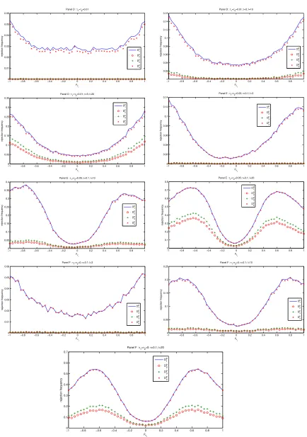
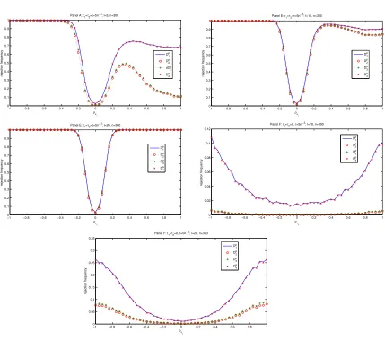
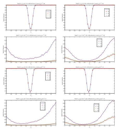
may still have power as long asΠ0ρυu6= 0 [see Panels(B)&(C)in Figure 1]. In the other side, if

Π0ρ_{υu 6}= 0, the power of all tests is low even whenθis identified or close so [as an illustration of

this, see Panel(D)in Figure 1]. We now study in Section 3.3, the behaviour of the tests in a Monte

Carlo experiment.

3.3. Size and power comparison

We consider the following data generating process (DGP):

y = Y1β1+Y2β2+W θ+u ,

(Y1, Y2, W) = Z(Π1,Π2,Γ) + (υ1, υ2, ξ), (3.3)

whereY = [Y1, Y2] is a n×2matrix of regressors of interest. W (here an×1vector)8 is the

endogenous variable which exogeneity is not being tested.Z containslinstruments each generated

i.i.dN(0,1) and is kept fix within experiment. So,Π1, Π2 andΓarel-dimensional vectors.

The errors(u, υ1, υ2, ξ)are generated such that:

ui = (1 +ρ2υ1+ρ

2

υ2+ρ

2

ξ)−1/2(ε1i+ρυ1ε2i+ρυ2ε3i+ρξε4i),

υ1i = (1 +ρ2υ1)

−1/2_(ρ

υ1ε1i+ε2i), υ2i = (1 +ρ

2

υ2)

−1/2_(ρ

υ2ε1i+ε3i),

ξ_i = (1 +ρ2_ξ)−1/2(ρ_ξε1i+ε4i),(ε1i, ε2i, ε3i, ε4i)′i.i.d∼ N(0, I4) (3.4)

for all i = 1, . . . , n, ₋1 _≤ ρ_{υ1 ≤} 1, ρ_υ2 = ρ_υ1/√3, and ρ_ξ is kept at ρ_ξ = 0.8. From this parametrization, the partial null exogeneity ofY is then expressed as Hp₀ : ρ_υ1 = 0. As seen from (3.4),ξis not correlated with(υ1, υ2)under Hp0, but is under the alternative hypothesis. To extend

the model to cases where ξ is locally correlated with (υ1, υ2), as required Assumption 2.4, we weakened the non correlation assumption between ξ and (υ1, υ2). The results for this setup are

presented in Figure 5 of Appendix B. They indicate that the tests are still valid even for moderate

correlation betweenξand(υ1, υ2).

The values ofβ₁, β₂ andθare set at2, ₋3 and1/2, respectively. Π1, Π2 andΓ are chosen

as: Π1 = τ1Π01, Π2 = τ2Π02, Γ = τΓ0, where [Π01,Π02,Γ0]is obtained by taking the

first three columns of the identity matrix of dimension l. To account for strong, partial and weak

identification of model parameters, we consider six panels for the values ofτ1,τ2andτ as follows:

(A) τ1 = τ2 = τ = 5, i.e. β1, β2 and θ are identified; (B) τ1 = τ2 = 5, τ = 0, so, β1

and β₂ are identified but θ is not (partial identification); (C)τ1 = 5, τ2 =τ = √0.1_n, i.e. β1 is

identified butβ₂ andθ are weakly identified; (D) τ1 =τ2 = √0.1_n, τ = 5, henceθ is identified

but β₁ and β₂ are weakly identified; (E) τ1 = τ2 = √0._n5, τ = √1_n, i.e., all model parameters

are weakly identified; and finally (F) τ1 = τ2 = 0, τ = √1_n : β1 and β2 are completely non

identified (irrelevant instruments), andθis weakly identified. The number of instruments lbelong

to_{3,10,20_}. Since we havem = 3 endogenous regressors in (3.3), l = 3 corresponds to the

usual “just-identified” setup, whilel > 3 corresponds to the “overidentification”. The simulations

are run with sample sizes100 and 300,while the number of replications is N = 10,000. In all

cases, the nominal level is set at5 %.

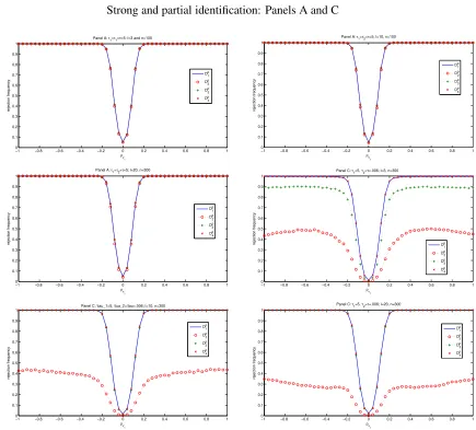
Figures 1- 2 presents the power curves of the tests forn= 100,while Figures 3-4 in Appendix

B is for n = 300. The results are qualitatively the same in terms of level control in both cases.

However, the power improves substantially whenn= 300,as expected. First, we observe that all

tests have correct level whether identification is strong, partial or weak. Furthermore,Dp

1 and D

p

4

have approximately a good level even when IVs are weak [for example, see Figure 2 below and

Figure 4 in Appendix B where identification is weak]. However, the same figures show clearly that

Dp

2andD3pare overly conservative. In the same vain, all tests have similar power when identification is strong strong (see Panel(A)in Figure 1& 3), butDp

1 andD

p

4 exhibit more power thanD

p

Dp

3 when identification is partial or weak. In addition, the results confirm that the tests have power

when the parameter of the regressors which exogeneity is tested (hereβ) is identified (for example,

see Panel(B)&(C)in Figure 1). But power is low whenβ is weakly identified, even whenθis

strongly identified (see Panel(D)Figure 1). Overall, the recommendation is to use the testsDp

1 and

Dp

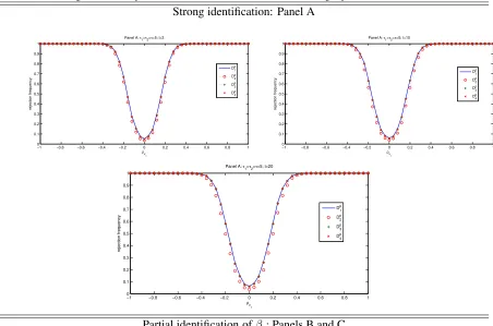
Figure 1. Size and power at nominal level5%when identification is strong or partial,n= 100 Strong identification: Panel A

−10 −0.8 −0.6 −0.4 −0.2 0 0.2 0.4 0.6 0.8 1 0.1 0.2 0.3 0.4 0.5 0.6 0.7 0.8 0.9 1

ρv1

rejection frequency

Panel A: τ1=τ2=τ=5; l=3

D 1 p D 2 p D3 p D 4 p

−1 −0.8 −0.6 −0.4 −0.2 0 0.2 0.4 0.6 0.8 1 0 0.1 0.2 0.3 0.4 0.5 0.6 0.7 0.8 0.9 1

ρv1

rejection frequency

Panel A: τ1=τ2=τ=5; l=10

Dp 1 Dp 2 Dp 3 Dp 4

−1 −0.8 −0.6 −0.4 −0.2 0 0.2 0.4 0.6 0.8 1 0 0.1 0.2 0.3 0.4 0.5 0.6 0.7 0.8 0.9 1

ρv1

rejection frequency

Panel A: τ₁=τ₂=τ=5; l=20

D₁p

D₂p

D₃p

D₄p

Partial identification ofβ :Panels B and C

−10 −0.8 −0.6 −0.4 −0.2 0 0.2 0.4 0.6 0.8 1 0.1 0.2 0.3 0.4 0.5 0.6 0.7 0.8 0.9 1 ρv 1 rejection frequency

Panel B: τ1=τ2=5; τ=0; l=3

Dp 1 Dp 2 Dp 3 Dp 4

−1 −0.8 −0.6 −0.4 −0.2 0 0.2 0.4 0.6 0.8 1 0 0.1 0.2 0.3 0.4 0.5 0.6 0.7 0.8 0.9 1 ρv 1 rejection frequency

Panel B: τ1=τ2=5; τ=0; l=10

Dp 1 Dp 2 Dp 3 Dp 4

−10 −0.8 −0.6 −0.4 −0.2 0 0.2 0.4 0.6 0.8 1 0.1 0.2 0.3 0.4 0.5 0.6 0.7 0.8 0.9 1

ρv1

rejection frequency

Panel B: τ1=τ2=5; τ=0; l=20

Dp 1 Dp 2 Dp 3 Dp 4

−1 −0.8 −0.6 −0.4 −0.2 0 0.2 0.4 0.6 0.8 1 0 0.1 0.2 0.3 0.4 0.5 0.6 0.7 0.8 0.9 1

ρv1

rejection frequency

Panel C : τ1=5; τ2=τ=0.01

Dp 1 Dp 2 Dp 3 Dp 4

−10 −0.8 −0.6 −0.4 −0.2 0 0.2 0.4 0.6 0.8 1 0.1 0.2 0.3 0.4 0.5 0.6 0.7 0.8 0.9 1 ρ rejection frequency

Panel C : τ1=5; τ2=τ=0.01

Dp 1 Dp 2 Dp 3 Dp 4

−1 −0.8 −0.6 −0.4 −0.2 0 0.2 0.4 0.6 0.8 1 0 0.1 0.2 0.3 0.4 0.5 0.6 0.7 0.8 0.9 1 ρ rejection frequency

Panel C : τ1=5; τ2=τ=0.01; l=20

Figure 2. Size and power at nominal level5%when identification is weak,n= 100

Partial identification ofθand complete weak identification of all parameters: Panels D, E and F

−10 −0.8 −0.6 −0.4 −0.2 0 0.2 0.4 0.6 0.8 1 0.01 0.02 0.03 0.04 0.05 0.06

ρv1

rejection frequency

Panel D : τ1=τ2=0.01

Dp 1 Dp 2 Dp 3 Dp 4

−1 −0.8 −0.6 −0.4 −0.2 0 0.2 0.4 0.6 0.8 1 0 0.02 0.04 0.06 0.08 0.1 0.12 0.14 0.16

ρv1

rejection frequency

Panel D : τ1=τ2=0.01; τ=5; l=10

Dp 1 Dp 2 Dp 3 Dp 4

−10 −0.8 −0.6 −0.4 −0.2 0 0.2 0.4 0.6 0.8 1 0.05 0.1 0.15 0.2 0.25 0.3 0.35

ρv1

rejection frequency

Panel D : τ1=τ2=0.01; τ=5; l=20

Dp 1 Dp 2 Dp 3 Dp 4

−1 −0.8 −0.6 −0.4 −0.2 0 0.2 0.4 0.6 0.8 1 0 0.02 0.04 0.06 0.08 0.1 0.12 0.14

ρv1

rejection frequency

Panel E : τ1=τ2=0.05; τ=0.1; l=3

Dp 1 Dp 2 Dp 3 Dp 4

−10 −0.8 −0.6 −0.4 −0.2 0 0.2 0.4 0.6 0.8 1 0.05 0.1 0.15 0.2 0.25 0.3 0.35 0.4

ρv1

rejection frequency

Panel E : τ1=τ2=0.05; τ=0.1; l=10

Dp 1 Dp 2 Dp 3 Dp 4

−1 −0.8 −0.6 −0.4 −0.2 0 0.2 0.4 0.6 0.8 1 0 0.1 0.2 0.3 0.4 0.5 0.6 0.7 0.8

ρv1

rejection frequency

Panel E : τ1=τ2=0.05; τ=0.1; l=20

Dp 1 Dp 2 Dp 3 Dp 4

−1 −0.8 −0.6 −0.4 −0.2 0 0.2 0.4 0.6 0.8 1 0 0.01 0.02 0.03 0.04 0.05 0.06

ρv1

rejection frequency

Panel F : τ1=τ2=0; τ=0.1; l=3

Dp 1 Dp 2 Dp 3 Dp 4

−1 −0.8 −0.6 −0.4 −0.2 0 0.2 0.4 0.6 0.8 1 0 0.05 0.1 0.15 0.2 0.25

ρv1

rejection frequency

Panel F : τ1=τ2=0; τ=0.1; l=10

Dp 1 Dp 2 Dp 3 Dp 4

−1 −0.8 −0.6 −0.4 −0.2 0 0.2 0.4 0.6 0.8 1 0 0.1 0.2 0.3 0.4 0.5 0.6 0.7 ρ_v 1 rejection frequancy

Panel F : τ1=τ2=0; τ=0.1; l=20

4.

Empirical illustration

We consider the return to education model from Card (1995) in Example2.1. The first-stage

speci-fications foreducand(exper, exper2_{) are given by}

educi = Z′Π+Z1′iδ1+υi,(experi, exper2i) =Zi′Γ+Z1′iδ1+ξi, i= 1, . . . , n (4.1)

whereZ1 and Z are the same as in (2.4). In Example2.1, we found that DWH-tests rejected the

joint exogeneity of(educ, exper, exper2), but we do not know if some regressors are exogenous.

In this application, we want to test the exogeneity of educ and (exper, exper2) separately. So,

two null hypotheses are considered: (i) Hp₀ : cov(υi, ui) = 0 for all i(partial exogeneity of

educ) and (ii) Hp₀ : cov(ξ_i, ui) = 0 for alli[partial exogeneity of (exper, exper2)], where u

is the structural error term in (2.4). Note that in the setup for(i), ξmay be correlated withu [i.e.

(exper, exper2_{) may be endogenous], while in those for (ii), υ may be correlated with u (i.e.}

educmay be endogenous).

Table 1 reports the outcomes of the DWH-tests and the Dp _{tests proposed in this paper. The}

DWH-tests are run under the assumption that the regressors not being tested are exogenous, while

theDp_{tests do not require this questionable restriction. It is important to observe that becauseexper}

is generated as exper = qge₋6₋educ, we havecov(experi, ui) = −cov(educi, ui), asage

is exogenous. So, any valid procedure that rejects the partial exogeneity ofeducshould also reject

those ofexper.This is not however the case for the DWH-tests, as they all fail to rejected the partial

exogeneity of (exper, exper2). This result is not surprising because educ is likely endogenous

and DWH procedures do not account for that when testing the exogeneity of (exper, exper2_).

The outcomes of the Dp _{tests indicate strong evidence against the exogeneity of both educ and}

(exper, exper2_{)as showed Table 1. Overall, these results underscore: (1) how the use of DWH}

tests to assess partial exogeneity hypotheses may be misleading, and(2)the relevance of usingDp

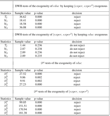
Table 1. Testing for partial exogeneity ofeducand(exper, exper2₎

DWH-tests of the exogeneity ofeduc by keeping(exper, exper2_)exogenous

Statistics Sample value p-value decision

T2 36.62 0.000 reject

H1 18.41 0.000 reject

H2 18.58 0.000 reject

H3 36.08 0.000 reject

DWH-tests of the exogeneity of(exper, exper2_{) by keepingeduc exogenous}

Statistics Sample value p-value decision

T2 1.44 0.236 do not reject

H1 2.87 0.238 do not reject

H2 2.89 0.236 do not reject

H3 2.89 0.235 do not reject

Dp_{-tests of the exogeneity ofeduc}

Statistics Sample value p-value decision

D₁p _{27.52 0.000 reject}

D₂p _{9.86 0.002 reject}

Dp

3 9.91 0.002 reject

Dp

4 27.23 0.000 reject

Dp_{-tests of the exogeneity of(exper, exper}2₎

Statistics Sample value p-value decision

Dp

1 99.05 0.000 reject

Dp

2 151.51 0.000 reject

D₃p _{170.94 0.000 reject}

5.

Conclusion

In this paper, we propose alternative tests for assessing partial exogeneity in a linear IV regression.

The tests are easy to implement as they only require OLS and IV regressions. We provide an

analysis of their asymptotic behaviour (level and power) which shows that all tests are valid (level

is controlled) whether model parameters are identified or not. So, the proposed tests robust to weak

instruments. Moreover, our analysis indicates that test consistency may still hold over a wide range

of cases where the overall identification fails, provided partial identification is satisfied. However,

all tests have low power when model parameters are completely not identified.

A Monte Carlo experiment confirms our theoretical results. We illustrate our theoretical finding

through the workhorse example of returns to education from Card (1995). Our results clearly

indi-cate that standard exogeneity tests of the type proposed by Durbin (1954), Wu (1973, 1974), and

Hausman (1978) are not appropriate to assess partial exogeneity hypotheses, as they are valid only

when the regressors not being tested are exogenous. For example, we find these tests fail to rejected

the exogeneity of experience variables in this model if education is assumed exogenous. In contrast,

all proposed tests in this paper find strong evidence against the exogeneity of both education and

ex-perience variables, separately. Overall, this application underscores the relevance of usingDp_-tests

APPENDIX

A.

Proofs

PROOF OFLEMMA2.5 Assume that rank(ΠY W) =m. First, writeu˜anduˆ∗as:

˜

u = u+ (W −W˜)θ=u+MZξθ+ ˆσθPZuˆ∗,uˆ∗=MX¯u∗=MX¯u+MX¯MZξθ (A.1)

whereX¯ = [Y,W¯]andˆσθ = ˆσuξθ/σˆ2u. Hence, we haveZ′u/n˜ = Z′u/n+ ˆσθZ′uˆ∗/n andZ′uˆ∗/n=

Z′_M¯

Xu/n +Z′MX¯MZξθ/n. When Assumptions 2.2-2.4 are satisfied and if further H0 holds, then ¯

X′_u/n→p _(σ′

υu,0)′= 0 and

¯

X′_X/n¯ p

→Q_X¯ = 



Π′_Q

ZΠ+Συ Π′QZΓ

Γ′_Q

ZΠ Γ′QZΓ



>0, Z′X/n¯

p

→QZX¯ =

QZΠ QZΓ

.

This then implies thatZ′_M¯

Xu/n=Z′u/n−(Z′X/n¯ )( ¯X′X/n¯ )−1( ¯X′u/n)

p

→0. Sinceυ′_ξ/n→p _0from Assumption2.4-(a), we also getZ′_M¯

XMZξθ/n

p

→0 so thatZ′_uˆ

∗/n=Z′M_X¯u/n+Z′M_X¯MZξθ/n p

→0.

So, we haveσˆuξ = ˆu′_∗W/(n−m)−(ˆu′_∗Z/n)(Z′Z/n)−1(ZW/(n−m)) = ˆu′_∗W/(n−m) +op(1) p

→

σ∗

uξ =σuξ+θ′Σξandσˆ2u

p

→σ∗2

u =σ2u+σuξθ.From Assumption2.4-(b), we haveσuξ =−θ′Σξso that

σ∗

uξ = 0andσ∗

2

u =σ2u−θ′Σξθ >0(by Assumption2.2). Hence, we haveσˆθ = ˆσuξθ/ˆσ2u p

→σθ= 0and

Z′_{u/n˜ =Z}′_{u/n+ ˆσ}

θZ′uˆ∗/n

p

→0.We shall now show thatW˜′_{u/n˜ →}p _0andY′_{u/n˜ →}p _{0. Observe first} thatW˜′_{u/n˜ = ˜Γ}′_Z′_{u/n.˜ SinceΓ}˜ _→p _{Γ, and from (??)Z}′_{u/n˜ →}p _{0, we haveW}˜′_{u/n˜ →}p _{0.By the same} way, we getY′_{u/n˜ =Y}′_(u+M

Zξθ+ ˆσθPZuˆ∗)/n

p

→συu. Asσυu= 0under Assumption H0, it is clear thatY′_{u/n˜ →}p _{0. The proof is similar for weak values ofΠ}

Y W, i.e.,ΠY W = √1_n[Π0,Γ0].

PROOF OFLEMMA 2.6 Firstly, from Lemma2.6, we have˜u=u+MZξθ+ ˆσθPZuˆ∗ = u+MZξθ+

PZPuˆ∗W θ+op(1), wherePuˆ∗ = ˆu∗(ˆu′∗uˆ∗)−1uˆ′∗ is the projection matrix in the space spanned by the residualsuˆ∗.So, we can writeZ⊥

′ ˜

u⊥_/√_nandυ⊥′_u˜⊥_/√_nas:

Z⊥′ ˜

u⊥_/√_{n = Z}⊥′

u⊥_/√_n+Z⊥′

MZξθ/√n+Z⊥

′

PZPuˆ∗W θ/

√

n (A.2)

υ⊥′_u˜⊥_/√_{n = υ}⊥′_u⊥_/√_n+υ⊥′_M

Zξθ/√n+υ⊥

′

PZPuˆ∗W θ/

√

n. (A.3)

Observe thatZ⊥′_M

Z =Z′MZ = 0andυ⊥

′

(A.2)-(A.3) become:

Z⊥′ ˜

u⊥_/√_{n = Z}⊥′

u⊥_/√_n+Z⊥′

PZPuˆ∗W θ/

√

n (A.4)

υ⊥′_u˜⊥_/√_{n = υ}⊥′_u⊥_/√_n+υ⊥′_P

ZPuˆ_∗W θ/√n+op(1). (A.5)

As Z′_uˆ

∗/n = op(1), υ⊥

′

Z/n = op(1) and uˆ′_∗W/√n = Op(1), we have υ⊥

′

PZPuˆ∗W θ/

√

n = (υ⊥′_Z/n)(Z′_Z/n)−1_)(Z′_uˆ

∗/n)(ˆu′∗uˆ∗/n)−1(ˆu′∗W/

√

n) = 0p(1). Moreover, sinceΓ˜ p

→ Γ (withΓ = 0

when ΠY W = √1_n[Π0,Γ0]), we have υ′W /n˜ = (υ′Z/n)˜Γ

p

→ 0 so that υ⊥′_u⊥_/√_{n = υ}′_u/√_n− (υ′_{W /n}˜ _{)( ˜W}′_{W /n}˜ ₎−1_Γ˜(Z′_/√_{n) = υ}′_u/√_n+o

p(1). By the same way, we getZ⊥

′

PZPuˆ∗W θ/

√

n = (Z⊥′_Z/n)(Z′_Z/n)−1_)(Z′_uˆ′

∗/n)(ˆu′∗uˆ∗/n)−1(ˆu′∗W θ/

√

n) =op(1) so that we can express (A.4)-(A.5) as:





Z⊥′_u˜⊥_/√_n

υ⊥′_u˜⊥_/√_n 

 = 



A1n 0

0 Imy



 



Z′_u/√_n

υ′_u/√_n 

+op(1) (A.6)

where A1n = Il − (Z′Z/n)Γ˜(Γ˜′(Z′Z/n)Γ˜)−1Γ˜′ and





Z′_u/√_n

υ′_u/√_n   d →   ψZu ψυu   ∼ N 

0, σ2_u 



QZ 0

0 Συ



 

by Assumption2.3. We shall now distinguish two cases:(1)rank(ΠY W) =m,

and(2)ΠY W = √1_n[Π0,Γ0].

(1) Suppose first that rank(ΠY W) = m. Then, A1n p

→ A1 = Il − QZΓ(Γ′QZΓ)−1Γ′ =

Q1Z/2MQ1Z/2ΓQ

−1/2

Z and from (A.6) we have





Z⊥′ ˜

u⊥_/√_n

υ⊥′ ˜

u⊥_/√_n   d →  

ψZ⊥_u˜

ψυ⊥u˜ 

= 



Q1Z/2MQ1Z/2ΓQ

−1/2

Z 0

0 Imy

    ψZu ψυu   ∼ N 

0, σ2_u 



QZ⊥ 0 0 Συ



 

, QZ⊥ =Q

1/2

Z MQ1Z/2ΓQ

1/2

Z .

(2) Suppose now that ΠY W = √1_n[Π0,Γ0] and write √nΓ˜ = Γ0 + (Z′Z/n)−1(Z′ξ/√n)− ˆ

σθ(Z′Z/n)−1(Z′uˆ∗/√n). From the proof in Lemma 2.5, we haveσˆθ = ˆσuξθ/σˆ2u p

→ σθ = 0. From

Assumption 2.3, we also have (Z′_Z/n)−1_(Z′_ξ/√_{n) →}d _Q−1

Z ψZξ. We now focus on Z′uˆ∗/√n. Let us decomposeMX¯ asMX¯ =MW¯ −PMW¯Y and writeZ

′_uˆ

∗/√nas:

Z′uˆ∗/

√

n=Z′M_X¯u_∗/√n = Z′M_W¯u_∗/√n−(Z′M_W¯Y /n)(Y′M_W¯Y /n)−1(Y′M_W¯u_∗/√n)

= [Il−(Z′M_W¯Y /n)(Y′M_W¯Y /n)−1Π′]Z′M_W¯u_∗/√n+

Since Z′_M¯

Wu∗/√n = [Il − (Z′Z/n)Γˆ(Γˆ′(Z′Z/n)Γˆ)−1Γˆ′]Z′u∗/√n = [Il −

(Z′_Z/n)Γˆ_(Γˆ′_(Z′_Z/n)Γˆ₎−1_Γˆ′_]Z′_u/√_{n and υ}′_u

∗/√n = υ′u/√n+υ′MZξθ/√n = υ′u/√n+op(1)

[becauseυ′_M

Zξθ/√n=op(1)under H0], we can express (A.7) as:

Z′_uˆ ∗/

√

n = A2nZ′u/√n+A3nυ′u/√n+op(1) (A.8)

where A2n = [Il −(Z′M_W¯Y /n)(Y′M_W¯Y /n)−1Π′][Il −(Z′Z/n)Γˆ(Γˆ′(Z′Z/n)Γˆ)−1Γˆ′] and A3n =

(Z′_M¯

WY /n)(Y′MW¯Y /n)−1. As ΠY W = √1_n[Π0, Γ0], we find: Z′M_W¯Y /n →p 0 Y′M_W¯Y /n →p

Συ, A2n p

→ A2 = Q1_Z/2M_Q1/2

Z ΓξQ

−1/2

Z where Γξ = Γ0 + Q−

1

Z ψZξ, and A3n

p

→ 0. Hence, we get and Z′_uˆ

∗/√n

d

→ Q1Z/2MQ1Z/2ΓξQ

−1/2

Z ψZu and

√

nΓ˜ _→d Γ(ψZξ) = Q−

1/2

Z (Q

1/2

Z Γξ −

σθM_Q1/2

Z ΓξQ

−1/2

Z ψZu) ≡ Γξ (since σθ = 0). Moreover, we have A1n →d A1 = Il −

QZΓ(ψZξ)(Γ(ψZξ)′QZΓ(ψZξ))−1Γ(ψZξ)′ =Q

1/2

Z MQ1Z/2Γ(ψZξ)Q

−1/2

Z and (A.6) then implies that





Z⊥′ ˜

u⊥_/√_n

υ⊥′ ˜

u⊥_/√_n   d →  

ψZ⊥_u˜

ψυ⊥_u˜



= 



Q1_Z/2M_Q1/2

Z Γ(ψZξ)Q

−1/2

Z 0

0 Imy

    ψZu ψυu 

. (A.9)

BecauseψZ⊥u˜=Q 1/2

Z MQ1Z/2Γ(ψZξ)Q

−1/2

Z ψZu, it is clear thatQ−

1/2

Z ψZ⊥u˜is independent ofQ 1/2

Z Γ(ψZξ).

Since QZ is fixed, ψZ⊥u˜ is also independent of Q 1/2

Z Γ(ψZξ). So, conditionally on Q

1/2

Z Γ(ψZξ) =

Q1_Z/2Γ(x2), (A.9) implies that





ψZ⊥_u˜

ψυ⊥_u˜



|_Q1/2

Z Γ(x2)∼N h

0, σ2udiag(Q

1/2

Z MQ1/2

Z Γ(x2)Q 1/2

Z , Συ)

i

. (A.10)

By integrating (A.10) with respect to all possible realization ofψZξ, the result follows.

PROOF OFLEMMA3.1 (i)Assume first thatσυu= 0.We have

ˆ

βLS−β˜IV = (Y⊥

′

Y⊥_/n)−1_Y⊥′_u˜⊥_/n−(Y⊥′_P

Z⊥Y⊥/n)−1Y⊥

′

PZ⊥u˜⊥/n,

√

n(ˆβLS−˜βIV) = (Y⊥

′

Y⊥_/n)−1_Y⊥′ ˜

u⊥_/√_n−(Y⊥′

PZ⊥Y⊥/n)−1Y⊥ ′

PZ⊥u˜⊥/√n,

Y⊥′_Y⊥_{/n = Y}′_{Y /n−(Y}′_Z/n)√_nΓ˜_[√_nΓ˜′_(Z′_Z/n)√_nΓ˜_]−1√_nΓ˜′_(Z′_{Y /n),}

Y⊥′

PZ⊥Y⊥/n = (Y′M_W˜Z/n)(Z′M_W˜Z/n)−1(Z′M_W˜Y /n),

Y⊥′_u˜⊥_{/n = Y}′_{u/n˜ −(Y}′_{W /n}˜ _{)( ˜W}′_{W /n}˜ ₎−1_{( ˜W}′_{u/n˜ ),}

Y⊥′