The product life cycle of durable goods

The product life cycle of durable goods

Kaldasch, Joachim

EBC Hochschule Berlin

September 2011

Online at

https://mpra.ub.uni-muenchen.de/66582/

The Product Life Cycle of Durable Goods

Joachim Kaldasch

EBC Hochschule Berlin

Alexanderplatz 1, 10178 Berlin, Germany

(Email: joachim.kaldasch@international-business-school.de)

Abstract

A dynamic model of the product lifecycle of (nearly) homogeneous durables in polypoly markets is established. It describes the concurrent evolution of the unit sales and price of a good. The theory is based on the idea that the sales dynamics is determined by a meeting process of demanded with supplied product units. Taking advantage from the Bass model for first purchase and a logistic model for repurchase the entire product lifecycle of a durable can be established. For the case of a fast growing supply the model suggests that the mean price of the good decreases according to a logistic law. Both, the established unit sales and price evolution are in agreement with the empirical data studied in this paper.

The presented approach discusses further the interference of the diffusion process with the supply dynamics. The model predicts the occurrence of lost sales in the initial stages of the lifecycle due to supply constraints. They are the origin for a retarded market penetration. The theory suggests that the imitation rate B indicating social contagion in the Bass model has its maximum magnitude for the case of a large amount of available units at introduction and a fast output increase. The empirical data of the investigated samples are in qualitative agreement with this prediction.

1. Introduction

A microeconomic model is presented that investigates the product lifecycle (PLC) of (nearly) homogeneous durables in polypoly markets.1 The product lifecycle concept suggests that analogous to the life of organisms goods are subject to characteristic stages in their unit sales evolution classified usually into introduction, growth, maturity and decline phase [1]. The PLC of durables was studied intensively in order to forecast the adopter and sales evolution [2-4]. It also applies as a guideline for corporate marketing strategy and in operation research in order to estimate production capacities [5-7].

The unit sales evolution is determined by first- and repurchase of a durable. First purchase is related to the spreading of a good into the market. Repurchase is proportional to the number of current adopters and a corresponding repurchase rate that describes multiple and replacement purchase of product units. The evolution of the market penetration is known as market diffusion stipulating the initial stages of the PLC. In particular the Bass model turned out to give an appropriate picture of the diffusion process of consumer durables [8]. It suggests that the market diffusion of new products consists of a fast and a slow spreading wave. The fast wave is mediated by mass media and the slow one is due to social contagion. While diffusion models work well as a forecast tool the implementation of the price as a decision variable turned out to be difficult. A variety of models based on the Bass model were developed in order to include the price. It is usually taken into account as a perturbation of the spreading process [4,9,10]. The price, though, is a key microeconomic variable that has its origin in the relation between supply and demand. The presented dynamic model offers an alternative approach to understand the unit sales and price evolution not only of durables but also of non-durable goods in a unique framework [11].

The key idea to combine the sales and price dynamics of a durable is to treat purchase events as a meeting process of demanded (required) and supplied (available) product units. While the spreading process determines the generation rate of demanded units, the number of available units is a result of the output of suppliers. Their evolution determines the price of the good. It can be shown that based on this idea the price dispersion of homogeneous goods has for short time periods the form of a Laplace distribution [12,13]. The mean price of this distribution is determined by a Walrus equation. It suggests that an excess growth of demanded units cause an increase and an excess growth of supplied units a decrease of the mean price [14]. The presented model is an application of these considerations and rigorously derives the PLC of durable goods from the dynamics of demand and supply.

The paper is organized as follows. The next section establishes a model for the PLC of durables in polypoly markets. It starts with the derivation of the market dynamics of demanded and supplied product units followed by a consideration of the price dynamics of homogenous goods. After deriving the sales and price dynamics of durables the impact of the supply evolution on the rate of adoption is studied. The presented approach is applied to empirical investigations of the PLC of nearly homogenous consumer durables where market penetration and price data are available. The theory of the PLC of durable goods is summarized in the discussion, followed by the main conclusions of this work.

1

2. The Model

2.1. The Dynamics of Polypoly Markets

The model presented here is established for (nearly) homogeneous durable goods in polypoly markets. The demand side of the durable market is determined by the total number of demanded (desired) units ~x(t)at time step t generated by potential buyers. The supply side on the other hand is given by the total number of supplied (available) units~z(t)offered by N(t) suppliers (retailers). For a polypoly market we demand that N(t)>>1.

The total unit sales of the durable are indicated~y(t). As mentioned above the main idea of the presented microeconomic approach is to consider purchase events as the meeting of demanded and supplied product units. Therefore~y(t)must vanish if either ~x(t)or~z(t)

disappears. Hence the total unit sales can be written up to the first order as a product of both variables [15]2:

) ( ~ ) ( ~ ) (

~ _{t z t x t}

y 

(1)

where the unknown rate η characterizes the mean frequency by which the meeting process generates successful purchase events. Since~x(t),~z(t),~y(t)≥0, we demand that also η≥0. The evolution of the number of demanded and supplied units can be written as conservation relations of the form3:

) ( ~ ) ( ~ ) ( ~ t y t d dt t x d   (2) and ) ( ~ ) ( ~ ) ( ~ t y t s dt t z d   (3)

Eq.(2) suggests that the total number of demanded units increases with the total demand rate

) ( ~

t

d which represents the generation rate of demanded units by potential buyers. The number )

( ~ _t

x decreases in time by the purchase of product units with the total unit sales rate ~y(t). Eq.(3) states that the total number of supplied units increases by the supply of product units with the total supply rate (total output)~s(t)and decreases due to the purchase of these units with the total unit sales rate~y(t). The variables in Eq.(3) can be obtained in a polypoly market from a sum over the number of suppliers N(t) by:

2

Note that this form of relation has its origin in the description of chemical reactions in terms of rate equation, where the reaction rate is proportional to the product of their concentrations. This form was applied also to other meeting processes in physics, chemistry, biology and economy []. So for example the second term of the Bass model considered below has a similar form describing the meeting of potential adopters with current adopters. This approach is not applicable to the case of rare purchase events known for example from luxury goods.

3







~ N t

i i t N i i t N i

i t s t s t y t y t

z t

z

(4)

2.1.1. Demand and Supply

In order to establish the market evolution of a durable the dynamics of demand and supply has to be specified. We assume that demanded units do not last forever ones they are generated. Instead we take into account that they have a finite mean lifetime Θ. That means, demanded units not leading to purchase events during a time period Θ disappear. This effect can be included in the demand rate d~(t) by writing:

   ~( ) ~( ) ) ( ~ 0 t x t d t d (5)

where d~0(t) describes the generation rate of demanded units by potential buyers and the

second term takes the disappearance of demanded units with the rate 1/Θ into account. The amount of demanded units generated by the rate d~0(t) can be given by:

) ( ~ ) ( ~ 0

0 t d t

x 

(6)

The supply side is governed by the reproduction process. In a free market suppliers sell product units in order to make profit. Reinvesting a part of their profit and external money they can increase the total output~s(t) in time. This growth process can be characterized by the variable γ(t), defining the relation between total supply flow and total unit sales: 4

1 ) ( ~ ) ( ~ ) (   t y t s t  (7)

With this relation Eq.(3) turns into5:

) ( ~ ) ( ) ( ~ t y t dt t z d _

(8)

We want to confine here to fast growing markets with γ(t)>0. For a sufficiently high γ the number of supplied units evolves much faster than the number of demanded units in the considered time interval Δt such that:

4

This variable is also called reproduction parameter, since it characterizes the growth process of the output in the reproduction process.

5

dt t z d dt t x

d~( ) ~( )



(9)

In this case we can approximate:6

0 / ) (

~_{x t dt}

d

(10)

and obtain immediately from Eq.(2) and Eq.(5):

) ( ~ 1 ) ( ~ ) ( ~ ) ( ~

0 t x t

d t d t y     (11)

In this approximation the unit sales are equal to the generation rate of demanded units diminished by the rate ~x(t)/Θ. Applying Eq.(1) and Eq.(6) in Eq.(11) we get for the total number of demanded units:

) ( ~ 1 ) ( ~ ) ( ~ 0 t z t x t x     (12)

Expanding this relation for small ~z(t) yields:





) ( ~ ) ( ~

0 t z t

x t

x  

(13)

In order to determine the time evolution of ~z(t)we apply Eq.(13) in Eq.(1). Eq.(8) turns into:

2 ) ( ~ ) ( ) ( ~ ) ( ) ( ~ t z t t z t dt t z

d _{ }

(14) with: ) ( ~ )

(t x₀ t

 

(15)

In order to solve Eq.(14) we approximate the time dependent growth rate of supplied units

α(t) by its time average over the considered time interval Δt:



In this approximation Eq.(14) becomes a logistic differential equation with constant coefficients. The evolution of the number of supplied units can be given by:

t ze C z t

z _

  1 ) ( ~ max (17)

with the integration constant Cz and:

   1 max z (18)

The time evolution of the total number of available units depends on the sign of the supply growth rate α. For the considered supply market with α>0, Eq.(17) predicts that ~z(t)increases in time according to a logistic law until z(t)=zmax. Inserting zmax in Eq.(12) suggest that the

number of demanded units becomes ~x(t)~x₀(t)/2in the saturated state. This consideration is based on the condition that no supply constraints occur during Δt.7

The total unit sales Eq.(11) have with Eq.(12) and Eq.(17) the form:

t ze C t d z t z t d t

y _

   1 ) ( ~ ) ( ) ( ~ ) ( ~ 0 max 0 (19)

This relation suggests that the sales evolution is determined on the one hand by the generation rate of demanded units d~₀(t) and on the other hand by the evolution of available units ~z(t). At introduction of the good ~z(t) is necessarily small. Therefore the unit sales might be limited by the amount of available units. As a result these unsatisfied demands lead to lost sales.8 With an increasing supply flow this effect disappears.

2.1.2. The Mean Price Evolution of Homogeneous Goods

In order to take the product price p of the homogeneous good as a decision variable of potential buyers into account, we introduce the price dependent cumulated distribution functions of demanded and supplied units x(p,t) and z(p,t) by:

' ) ' , ( ' ) ( ~ ) , ( 0 dp p t x t x p t x p





If there are supply constrains the number of supplied units is bounded by a zmax that is smaller than given by

Eq.(18). In this case the supplied units evolve in logistic waves suggested by empirical data of durables discussed below.

8

where x’(p,t) and z’(p,t) are the probability densities to find demanded respectively supplied units in a given price interval p and p+dp. The functions x(p,t) and z(p,t) can be interpreted as demand and supply curves of the good. Generalizing Eq.(1) we assume that the number of sold units in a given price interval must disappear if the corresponding numbers of x(t,p) respectively z(t,p) vanish. Hence the price dependent unit sales are up to the first order proportional to both variables:

) , ( ) , ( ) ,

(t p x t p z t p

y 

(22)

where the meeting rate η is treated as price independent. The price dispersion of sold units of a homogeneous good is determined by the probability density Py(t,p) defined by:

 

(23)

As established in [12,13] the price dispersion of homogeneous goods can be derived from Eq.(22). For short time horizons the price dispersion has the form of a symmetric Laplace distribution:       p

y p e

P 2 1 ) ( (24)

with the standard deviation:









Std ( )  2  2  (25)

where μ is the mean price of the distribution and μm>0 is a minimum mean price indicating a

technological limit beyond which the supply of product units is not profitable. Further derived in these references is a relation that governs the dynamics of the mean price μ(t). It suggests that the mean price is determined by a Walrus equation of the form:

      _   dt z d dt x d H dt d m ~ ~ 1    (26)

where H>0 is a constant. This relation can be used to characterize the evolution of the mean price of homogeneous durables in the considered market constellation. For this purpose we take advantage from Eq.(10) and rewrite Eq.(26) as:

dt t z d H dt t d t _m ) ( ~ ) ( ) (

1 _



  

(27)





while higher order terms in~z(t)are neglected. For α>0 the mean price of a durable is declining in time due to the excess supply.9 The stationary solution of this relation is given either by μ=μm or ~z zmax. Eq.(25) suggests that for μ=μm the standard deviation disappears

and market becomes a monopoly market. Since we focus here on polypoly markets this case is not further considered.

For μ(t)>μm, Eq.(27) can be written as:





and we readily obtain:





m t z H t z H e

t    

       ) ( ~ 1 )

( ~() ₀

0

(30)

The model suggests that for a polypoly market the mean price declines with increasing~z(t)

given by Eq.(17). For ~z(t)z_maxthe mean price approaches a floor price μf>μm governed by

a logistic law. The floor price can be obtained from:

m

f  Hz 

  ₀exp( _max)

(31)

The introduction mean price of the good μ(0) is defined by:

m

z

H 



(0) ₀exp( ~(0))

(32)

while generally~z(0)0.

2.2. The Unit Sales Evolution

The evolution of the total unit sales of a good is usually referred to as product lifecycle. The total unit sales are the result of the first- and repurchase of the durable. First purchase is related to the spreading of the good into the market. This spreading process can be described by the cumulative number of adopters NA(t). In order to be in line with previous

research we want to define the market penetration n(t) by10:

M t N t

n_{( )} A( )

(33)

9

For α<0 the mean price would exhibit an exponential growth caused by a supply shortage.

10

The number of all possible adopters in a given domain interested in purchasing the consumer durable istermed market potential M.11

We want to take the inhomogeneity of the demand side of the market with respect to the price into account by introducing a market volume V(μ)≤M. It represents the number potential adopters who can afford the good for a mean price μ(t). The scaled market volume becomes:





M t V v() ( )

(34)

while 0≤v(μ)≤1. The market volume decreases with increasing mean price, dv(μ)/dμ<0. First purchase is determined by the time evolution of the number of adopters. This number is governed by a conservation relation and has the form:

) ( ) ( ) ( ) ( t n t t dt t

dn _{  }

(35)

The first term is the product of a generation rate φ(t) of adopters with the number of potential adopter ψ(t) not yet adopted the good. This variable can be written as the difference between the market volume and the current number of adopters:

) ( ) ( )

(t v  n t



(36)

The second term in Eq.(35) indicates the decline of n(t) with a mean decline rate θ. In the initial stages of the lifecycle is φ(t)>0, while θ≈0. The decline phase is characterized by

φ(t)≈0, θ>0. Expanding the generation rate φ(t) as a function of the number of adopters leads to:

) ( )

(t n t



(37)

with constant coefficients A, B>0. Inserting Eq.(37) in Eq.(35) with θ=0, we obtain a standard model for the spreading process of goods known as the Bass model [16]. The first purchase unit sales are determined by the growth of the market penetration:









) ( ) (

~ _{v n t n t v n t}

dt t dn t

yf        (38)

The Bass model suggests that the spreading of a good into a market consists of two waves. The first term indicates the fast wave due to the spontaneous purchase of potential adopters with the so-called innovation rate A. The second term indicates a slow spreading wave caused by social learning, where the number of adopters n(t) increases with an imitation rate B.

11

Repurchase events must be proportional to the current number of adopters. The total repurchased number of units per unit time ~yr(t) can therefore be modelled as the product of n(t) with a time dependent repurchase rate ξ(t) characterizing the average number of repurchased units per unit time and adopter:

) ( ) ( ) (

~ _{t t n t} y_r  (39)

The repurchase rate ξ(t) describes multiple and replacement purchase. Replacement purchase is due to the finite lifetime τ of the good caused for example by product failure. Multiple purchases can be specified by the number of units ι purchased during this mean lifetime. The repurchase rate ξ(t) approaches therefore after sufficient time to a maximum magnitude

ξmax=ι/τ.12 The growth of the repurchase rate up to ξmax can be modelled by the dynamic

equation:





d _{   }

(40)

where a>0 characterizes the growth rate of ξ(t). The solution of this relation determines the repurchase rate evolution:

at e C t _      1 ) ( max (41)

with the free parameter Cξ.

The total unit sales are the sum of first- and repurchase events:

) ( ) ( ) ( ) ( ~ ) ( ~ ) (

~ _{t n t}

dt t dn t y t y t

y  _f  _r  

(42)

The product lifecycle can be characterized by the main processes governing the adopter evolution:

i) In the introduction phase of the PLC the main source of the growth of n(t) is spontaneous purchase. Hence, the introduction phase is determined by the dominance of the first term in Eq.(38) over the second which leads to the condition A>Bn(t). It is related to the fast spreading wave of the good.

ii) In the growth phase social learning dominates the adopter evolution. This phase is related to the slow spreading wave where A<Bn(t) in Eq.(38). At the transition between both phases the number of adopters is ng≈A/B.

iii) In the maturity phase the spreading due to social contagion saturates while:

0 ) ( _ dt t dn (43) 12

Note that virtual goods like music, software or books have in infinite lifetime τ∞ and hence ξmax≈0.

From Eq.(38) follows with Eq.(43) that the number of adopters is determined in this period by: 0 ) ( )

(t v n

n   

(44)

The evolution of the market penetration n(t) can then be described by the solution of Eq.(38) given by: 0 2 ) ( ) ( 1 1 ) ( n e A B e t n t B A t B A              (45)

which yields an S-curve in time. The total first purchase unit sales caused by Bass diffusion become:









) ( 2 ) ( ) ( ~ _n Be A e B A A dt t dn t y t B A t B A

f _{ }

      (46)

However, according to Eq.(30) the mean price decreases in time and as a consequence the market volume v(μ(t)) increases. That means, when the spreading process due to social contagion slows down the number of potential adopters who cannot afford the good increases due to the decline of the mean price. This is an additional diffusion process related to the evolution of the mean price and the amount of adopters limited by their income. However, by studying the income distribution a peak in the income distribution is evident representing income limited potential adopters getting unemployment insurance or other social insurance income [].13 When the mean price declines such that these potential adopters can afford the good an additional second spreading wave is initiated in the maturity phase. It can be described by Eq.(38) as spontaneous purchase with A=A’, B=0 and the corresponding market volume n1.

iv) The decline phase is related to the occurrence of a close substitute of the current durable at time step td. This substitute changes the repurchase behaviour of potential buyers

immediately. For the case that the current good is ultimately replaced the repurchase rate ξ(t) declines in time while ξmax≈0. This effect can be taken into account in the time evolution of

the repurchase rate Eq.(40) by assuming a negative growth rate –a’. Eq.(40) turns therefore for t>td into:

) ( ' ) ( t a dt t

d _{ }

(47)

with a’>0 neglecting higher order terms in ξ(t). The differential equation has the solution:

13

  min ' ) ( ) (  

  a ttd 

d e

t t

(48)

where ξmin≈0 indicates a remaining minimum repurchase rate. As a result of the declining

repurchase rate the number of adopters declines with the rate θ>0. Applying Eq.(35) with

φ(t>td)=0 we get for t>td:

  min ) ( )

(t n t e n

n t td

d 

   (49)

while nmin is an eventually remaining minimum number of adopters.

The established relations allow a characterization of the entire product lifecycle for both, the evolution of the mean price and the unit sales and penetration evolution. In order to compare the model with empirical data a minimum set of free parameters is required. The evolution of ~z(t) entails three free parameters zmax, α and Cz. For the mean price evolution

four additional parameters are necessary μ0, μf, μm and H. The adopter evolution is

characterized here by Bass diffusion Eq.(45). It involves the free parameters A, B and n0, for

the second spreading wave at time step t1 the parameter A’ and n1.The decline phase starts at

td and requires two extra parameters θ and nmin. The total unit sales ~y(t) are governed by

Eq.(42) determined by Bass diffusion and the repurchase rate parameters a, ξmax and Cξ. The

decline phase finally uses the parameters a’ and ξmin. Since the empirical unit sales are usually

given in absolute numbers, for a comparison the market potential M has to be known. A complete description of the product lifecycle together with the mean price evolution involves a minimum number of 22 free parameters in the presented approximation.

2.3. The Relation between Market Penetration and Supply

Eq.(19) suggests that the initial stages of the lifecycle suffer from a constrained supply. This effect must have an impact on the velocity of the spreading process of a durable. Here we want to estimate the impact of a constrained supply on the imitation parameter B of the Bass model. For this purpose the total unit sales are approximated by the first purchase sales ~y_f(t) in Eq.(42). Further we can neglect the impact of spontaneous purchase on ~y_f(t)

since A≈0. From Eq.(19) follows with Eq.(38):

t ze C t d t t

n  _

   1 ) ( ~ ) ( ) ( 0 (50)

Obviously the impact of a constraint supply can be neglected if Cz=0. The idea is therefore to

treat the imitation parameter B as a function of Cz. Expanding B(Cz ) up to the first order

yields:

z

z B BC

C ) _{0 1}

(  



(51)

with the unknown coefficients B0 and B1. Inserting this relation in Eq.(50) and expanding also

the right hand side of Eq.(19) with respect to Cz we get:









z n t t d t Ce

C B

B₀ ₁ ( )( ) ~₀( )1 

(52)

A comparison of the coefficients leads to:

t e t d t t n B t d t t n

B₀ ( )( ) ~₀( ); ₁ ( )( )~₀( ) 

(53)

The relations suggest that B1 must be a time dependent function of the form:

t

e B t

B₁( ) ₀ 

(54)

Taking the time average over the growth period Δtg, we obtain for the mean magnitude of the

imitation parameter:











B tg t z g (55) with: z g t C t e g         1

(56)

Note that β≤0, because the exponential function is smaller than one for Δtg>0. Eq.(55)

suggests that B(β) is linear increasing function. The magnitude of the imitation parameter raises with increasing β until β=0. For β=0, the supply constraint has no impact on the imitation parameter. In this case B(β) has its maximum magnitude B0 and the diffusion

process takes place with maximum velocity. The diffusion is unperturbed for the case of a fast price decline related to a high α during the growth phase Δtg, respectively for small Cz

3. Comparison with Empirical Results

The presented model suggests that the PLC of (nearly) homogeneous consumer durables in polypoly markets have the following characteristics:

1. Homogeneous durable goods in polypoly markets have a price dispersion that can be approximated by the Laplace distribution Eq.(24).

2. For a fast growing supply the number of available units ~z(t)increases in time according to the logistic law Eq.(17). This evolution causes a logistic decline of the mean price described by Eq.(30).

3. Applying the Bass model for the market penetration n(t) the initial stages of the PLC can be approximated by Eq.(45) including a second spreading wave, while the decline phase is characterized by Eq.(49).

4. The total unit sales are determined on the one hand by the growth of the number of adopters and on the other hand by the repurchase of the good. The first purchase unit sales are given in the presented approximation by Eq.(46) as a result of the Bass model. Repurchase is determined by Eq.(39) with the logistic repurchase rate Eq.(41). The decline phase is governed by an exponential decay of the repurchase rate described by Eq.(48).

5. The diffusion processes is subject to a supply constraints causing a decelerated diffusion process. Plotting the imitation rate B as a function of β the model suggests a linear relationship of the form Eq.(55) .

In order to compare the presented model with available empirical data a number of consumer durables are studied satisfying the model conditions where the market penetration and the price evolution are known. For two samples also data of the empirical unit sales are available. Unfortunately the first assertion cannot be verified for the considered samples because the price dispersions of these goods are unknown. From empirical data of the price dispersion of homogeneous goods it was found, however, that their price dispersion can be approximated by a Laplace distribution [13,16,17]. It is assumed that the chosen examples exhibit similar distributions.

3.1. Market penetration, Mean Price and Supply Evolution

In order to illustrate the entire PLC of a durable, the empirical market penetration n(t) of Black & White (B&W) TV sets in the UK [18] is displayed in Fig.1 (squares) together with a fit of the Bass model Eq.(45) for the initial stages of the PLC (solid line) while Eq.(49) is applied for the decline phase. The fit parameters are summarized in Table 1 (solid line). Indicated are the phases characterizing the stages of the lifecycle as suggested by the model. The transition between introduction and growth phase takes place at a market penetration ng≈2%. The first spreading wave described by the Bass model in the maturity phase is

indicated by the dotted line. As expected, the decline phase of this good can be described by the exponential decay of the number of adopters by Eq.(49) starting at td=26 years. Displayed

in Fig.1 as a measure of the mean price μ(t) is the average sales price scaled by the maximum price [19]. The dashed line represents a fit of Eq.(30). Shown in the insert is the function ~z(t)

that follows from the fit of the mean price with the scaling zmax=1. According to this model

) (

~_{z t indicates the evolution of freely available units. Shown in Fig.2 is a similar example.}

summarized in Table 1. Unfortunately data for the decline phase of this durable are not available.

Presented in Fig.3 are the empirical market penetration and price evolution of CD-players in the USA [20]. This good has the smallest parameter α=0.17 in the considered collection of durables suggesting a slow increase of the total output in time. A consequence of the theory is that for small supply growth rates α the mean price is susceptible for demand and supply fluctuations. This can be seen in the initial period of the market penetration where a considerable fluctuation of the mean price is evident. Approaching the inflection point of the adopter evolution (maximum of the first purchase unit sales) price fluctuations settle down. A very fast growing market is that of DVD players in the USA displayed in Fig.4 [20]. This market has the highest supply growth rate α=0.65 exhibiting a rapid increase of supplied units accompanied with a considerable price decline.

Displayed in Fig.5 is the market evolution of Color TV sets in the USA [21]. Note that the Bass model applies merely up to about 80% of the total market potential. The presented model is derived for the case that ~z(t) does not suffer from supply constraints approaching zmax=1 with a constant supply growth rate α over the entire lifecycle Δt (Eq.(16)). The

empirical data suggest, however, that the supply evolution may have two separated logistic growth periods with zmax<1 and nearly constant α. In this case the price evolution can be

approximated by two logistic waves separated by time step t1. This result can be interpreted as

a rapid expansion of production capacities after introduction of the good followed by a much slower output increase. Applying two successive logistic waves the price and hence the supply evolution can be fitted with a higher accuracy. The data of the fit parameters αk,zmaxk,

Czk with k=0 for the first and k=1 for the second growth period are summarized in Table 1.

This supply evolution can be found also in the next two examples of durables. Shown in Fig.6 is the market evolution of cell phones in the USA [20]. The data suggest a considerable increase of the output up to t1=1991 accompanied by a rapid price decline. After

this growth period the expansion of the capacities slowed down. A dichotomy of the supply evolution is also evident in the market evolution of VCR’s in the USA [20] with two growth waves of nearly equal α.

3.2. The Unit Sales Evolution

In addition to the market penetration and price evolution the model allows also an investigation of the evolution of the total unit sales. For two examples empirical sales data are available. Displayed in Fig.8 are the total unit sales of VCR’s in the USA (squares) together with a fit of Eq.(46) and Eq.(39) for first- and repurchase (solid line) with the parameters given in Table 1 [20]. The model suggests that the sales peak with its maximum around 1986 is due to first purchase caused by Bass diffusion. The total unit sales growth until maximum magnitude was approached in 2000. The decline of the unit sales starts in 2001 caused by the introduction of DVD recorders as a close substitute.

Another example of the PLC of a consumer durable is displayed in Fig.9. It shows the rise and decline of the unit sales of CD-players in the USA (squares) and fit with the model equations (solid line) applying the parameters in Table 1 [20]. In difference to the VCR case the first sales peak due to the diffusion process in not clearly evident. This is due to the slow penetration of this good. The time until it is replaced by a close substitute (MP3 player) is much shorter than for VCR’s. The decline rate a’ for CD-Players is, however, much smaller

3.3. The Relation between Market Penetration and Supply

Eq.(55) predicts a linear relationship between the imitation parameter B of the Bass model as a measure of the diffusion velocity due to social contagion and the parameter β describing the impact of lost sales in the initial stages of the lifecycle. Taking advantage from the data in Table1 the relation between both parameters is plotted in Fig.10.14 From a linear regression fit we get for the solid line displayed in Fig.10 B0=1.7 and B1=1.1. Eq.(55)

suggests, however, that both parameters should be equal. Since this is not exactly the case and due to the small coefficient of determination (R2=0.8) of the regression fit we can conclude that the established theoretical considerations leading to Eq.(55) are qualitatively correct, but cannot verified quantitatively with this small number of examples.

4. Discussion

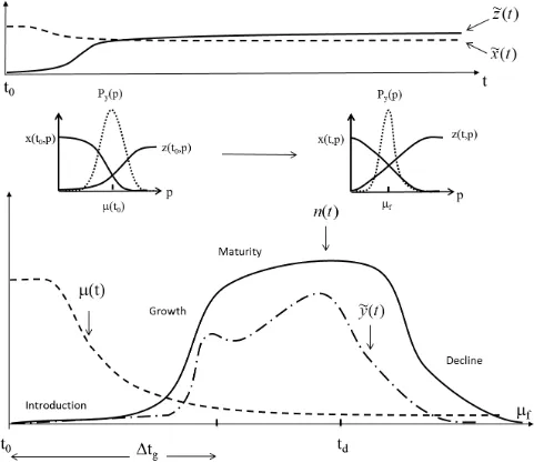
In this paper a dynamic microeconomic model of the PLC is established based on the dynamics of supply and demand. The PLC evolution is schematically displayed in Fig.11 for the case of a homogeneous durable in a fast growing polypoly market. At introduction of a new durable the total number of available units ~z(t) (solid line) is usually small compared to the corresponding total number of demanded units ~x(t)(dashed line). As a consequence not all demands can be satisfied. 15

The aggregated demand and supply curves x(t,p) and z(t,p) at the introduction time step t0 are indicated by solid lines in the right insert of Fig.11. The model is based on the idea

that sales events in a given price interval counted by the unit sales rate y(t,p) are the result of a meeting process of demanded and supplied product units given by the aggregated distribution functions x(t,p) and z(t,p). The chance that demanded and supplied product units meet is determined by the overlap of these functions. It has its maximum magnitude at the intersection point of x(t,p) with z(t,p). The unit sales y(t,p) and also the price dispersion Py(p)

have a maximum there and corresponds to the mean price μ(t) of the good. In similarity to the neo-classic microeconomic approach the market price is therefore determined by the intersection of the supply and demand curves.16 The resulting price dispersion Py(p) (dotted

line) has for homogeneous goods the form of a Laplace distribution.

For a fast growing output (a supply market) the functions x(t,p) and z(t,p) are subject to time-dependent variations inducing shifts of the mean price. The mean price evolution is governed by a Walrus equation, i.e. an excess increase of the number of demanded units increase and an excess increase of supplied units decrease the mean price in time. For the case of a fast supply growth the total number of available units ~z(t) increases in from of a logistic function until ~z(t)=zmax, while the number of demanded units ~x(t)declines in the run of time

indicated in the upper graph of Fig.11. As a result the mean price μ(t) declines governed by a logistic law approaching a floor price μf displayed in the lower graph of Fig.11 (For some

durables the empirical data suggest that this evolution takes place in form of two logistic waves). Note that the price dispersion does not only shift to lower values in the PLC, but

14

In the case of two supply waves, the data of the first wave with index 0 were taken.

15

Note that in this dynamic microeconomic model the unrealistic assumptions of the neo-classic model that all demanded units are necessarily equal to all supplied units can be omitted. Not satisfied demands disappear and do not contribute to the unit sales (Eq.(11)).

16

because a price is strictly positive Py(p) must become a narrow peak around the floor price μf

as schematically indicated in Fig.(11)[13].

Accompanied with the supply and demand evolution the good spreads into the market described here by Bass diffusion. The spreading process determines the evolution of the market penetration n(t) and first purchase sales. In order to complete the initial stages of the PLC repurchase is taken into account here by a logistic growth of the number of repurchased units per unit time.17 The decline phase of a good starts with the introduction of a close substitute at time step td. It has an impact on the repurchase behaviour of potential buyers

causing an exponential decline of the total unit sales and the number of adopters with time. The total PLC is schematically displayed in the lower graph of Fig.11 in terms of the total unit sales ~y(t)(dash-dot line) and market penetration n(t) (solid line). The characteristic stages of the lifecycle can be separated in this model by the main processes determining the adopter evolution also indicated in Fig.11.

Previous considerations suggested that the price evolution must have an impact on the diffusion process [22]. In the presented model a high introduction price would cause a small market volume. The declining mean price with increasing supply leads to a growth of the market volume. This additional price dependent diffusion process is not further discussed here (see [15]). But the mean price expresses also the relation between supply and demand. Explicitly derived in this paper is that a supply shortage in the initial stages of the PLC may cause lost sales. This effect is the origin of a decelerated spreading of the good. The imitation parameter B of the Bass model has its maximum magnitude for a fast growing supply during the growth period Δtg (high supply growth parameterα) and if the initial number of available

units is high (small Cz). A comparison with empirical investigations shows that the theoretical

considerations predicting a linear relationship between the imitation parameter B and a comprised parameter β indicating the supply growth are qualitatively correct.

5. Conclusions

We can conclude that:

1. The PLC of homogeneous durable goods in polypoly markets is determined by the complex dynamics of demand and supply. This dynamics generate a (Laplacian) price dispersion and governs the mean price evolution governed by a Walrus equation. While the demand side is characterized by the evolution first- and repurchase events the supply side is mainly determined by the output growth.

2. First purchase is related to the spreading process of the good into the market governed by a conservation relation for the number of adopters. The market penetration can be well described by the Bass model suggesting a fast and a slow spreading wave of the market penetration where the fast is mediated by mass media and the slow is due social contagion.

3. Repurchase is caused by the finite lifetime of a good and multiple purchase events. It can be modelled as a logistic growth of repurchase events.

4. The introduction of a close substitute changes the repurchase behaviour of potential buyers. It induces an exponential decline of the repurchase sales and market penetration.

5. Supply constraints in the initial stages of the PLC cause a retarded spreading of the good into the market. The imitation parameter of the Bass model decreases with a slow output growth and a small number of available units at introduction of the good.

17

References

[1] Chitale AK, Gupta R Product Policy and Brand Management. Prentice-Hall of India Pvt. Ltd.; 2010.

[2] Rogers EM. Diffusion of Innovations. Simon and Schuster, New York; 2003.

[3] Chandrasekaran D, Tellis GJ. A Critical Review of Marketing Research on Diffusion of New Products. Rev. Marketing Research. 2007; 3: 39-80.

[4] Peres R, Muller E, Mahajan V. Innovation diffusion and new product growth models: A critical review and research directions. Int. J. of Research in Marketing. 2010: 27: 91-106.

[5] Mahajan V, Muller E, Wind Y. New- Product Diffusion Models, Springer Verlag; 2000.

[6] Ho T-H, Savin S, Terwiesch C. Managing Demand and Sales Dynamics in New Product Diffusion under Supply Constraint. Managing Science. 2002: 48: 187-206.

[7] Hollensen S. Marketing Management. Pearson Education Ltd.; 2010. [8] Bass FM. A new product growth model for consumer durables.

Management Science. 1969; 15: 215-227.

[9] Feichtinger G. Optimal pricing in a diffusion model with nonlinear price dependent market potential. Operations Research Letters. 1982: 1: 236-240.

[10] Bass FM, Krishnan TV, Jain D. Why the Bass Model fits without Decision Variables. Marketing Science. 1994: 13: 203-223.

[11] Kaldasch J. Dynamic Model of Markets of Homogeneous Non-durables. British Journal of Economics, Management & Trade. 2015: 9: (3),1-12. Article no. BJEMT.19254.

[12] Kaldasch J. Evolutionary Model of Stock Markets. Physica A. 2014 ; 415: 449-462.

[13] Kaldasch J. Dynamic Model of the Price Dispersion of Homogeneous Goods. British Journal of Economics, Management & Trade. 2015: 8: Article no. BJEMT.2015.104.

[14] Zhang W-B. Synergetic Economics. Springer Verlag Berlin; 1991. [15] Kaldasch J. Evolutionary model of an Anonymous Consumer Durable

Market. Physica A. 2011; 390: 2692-2715.

[16] Kaplan G, Menzio G. The Morphology of Price Dispersion. 2015: NBER Working Paper No. 19877.

[17] Sapio S. An Empirically Based Model of the Supply Schedule in Day-Ahead Electricity Markets. LEM Working Paper Series. 2008; 13. [18] Harper R. Inside the Smart Home. Springer Verlag London; 2003. [19] Wang Z. Income Distribution, Market Size and the Evolution of

Industry. Review of Economic Dynamics. 2007: 11: 542-565.

[20] Coplan J. Diagnosing the DVD Disappointment: A life Cycle view. The Leonard N. Stern School of Business; 2006.

Available: http://w4.stem.nyu.edu/glucksman/docs/Coplan.pdf.

[21] Vanston LK. Practical Tips for Forecasting New Technology Adoption. Telektronikk. 2008: 3: 179-189.

Tables

Parameter B&W TV (UK)

B&W TV (USA)

CD Player

DVD Player

Colour TV

Cell Phone

VCR

Figure 1 2 3 4 5 6 7

t0 1946 1948 1983 1998 1954 1984 1978

α [ year-1

] 0.3 0.55 0.17 0.65 0.38 0.6 0.6

zmax 1 1 1 1

Cz 8 10 6 4

zmax0 0.28 0.5 0.5

Cz0 10 10 10

α0 [ year-1] 0.38 0.6 0.6

t1 [ years] 19 5 10

zmax118 0,72 0.5 0.5

Cz1 6 10 150

α1 [ year-1] 0.2 0.43 0.63

μ0 [%] 130 110 118 150 100 112 105

μf [%] 60 28.3 15 20 8 14 8

H 0.77 1.35 2.06 2 2.52 2 2.57

A [ year-1] 0.0065 0.05 0.0085 0.007 0.0005 0.0015 0.0018 B [ year-1] 0.4 0.4 0.45 1.2 0.4 0.55 0.64

n0 [%] 90 90 76 70 83 55 82

t1

A’

n1

M in Mio 85 79

td[ years] 26 17,8 23.8

θ[ year-1

] 0.16 nmin 0

a[ year-1] 0.3 0.31

a'[ year-1] 0.1 0.65

ξmin 0 0

ξmax 1.0 0.33

Cξ. 50 120

Δtg[ years] 20 14 18 10 25 15 16

β -1.03 -1.29 -1.25 -0.57 -1.02 -1,1 -1.03

Table 1. Characteristic parameters of the studied examples. For simplicity we have set μm=0.

18

Figures

Figure 1: Evolution of the market penetration n(t) (squares) and mean price μ(t) (triangles) of Black & White TV sets in the UK [18,19]. The solid line (market penetration) and dashed line (mean price) are a fit with the parameters in Table 1. The insert shows the function ~z(t)

Figure 7: Evolution of the market penetration n(t) (squares) and mean price μ(t) (triangles) of