www.hydrol-earth-syst-sci.net/18/2437/2014/ doi:10.5194/hess-18-2437-2014
© Author(s) 2014. CC Attribution 3.0 License.
Forchheimer flow to a well-considering time-dependent critical
radius
Q. Wang1, H. Zhan1,2, and Z. Tang1
1School of Environmental Studies, China University of Geosciences, Wuhan, Hubei, 430074, PR China 2Department of Geology and Geophysics, Texas A&M University, College Station, TX 77843-3115, USA Correspondence to: H. Zhan ([email protected])
Received: 11 October 2013 – Published in Hydrol. Earth Syst. Sci. Discuss.: 19 November 2013 Revised: 21 April 2014 – Accepted: 12 May 2014 – Published: 27 June 2014
Abstract. Previous studies on the non-Darcian flow into a pumping well assumed that critical radius (RCD)was a con-stant or infinity, where RCD represents the location of the interface between the non-Darcian flow region and Darcian flow region. In this study, a two-region model considering time-dependentRCDwas established, where the non-Darcian flow was described by the Forchheimer equation. A new iter-ation method was proposed to estimate RCD based on the finite-difference method. The results showed that RCD in-creased with time until reaching the quasi steady-state flow, and the asymptotic value of RCD only depended on the critical specific discharge beyond which flow became non-Darcian. A larger inertial force would reduce the change rate of RCD with time, and resulted in a smallerRCD at a spe-cific time during the transient flow. The difference between the new solution and previous solutions were obvious in the early pumping stage. The new solution agreed very well with the solution of the previous two-region model with a constant
RCDunder quasi steady flow. It agreed with the solution of the fully Darcian flow model in the Darcian flow region.
1 Introduction
Darcy’s law indicates a linear relationship between the fluid velocity and the hydraulic gradient (Bear, 1972), which is a basic assumption used to handle a great deal of problems re-lated to flow in porous and fractured media. However, many evidences from the laboratory and field experiments show that this linear law may be invalid in some situations, es-pecially when the groundwater flow velocity is sufficiently high or sufficiently low, where non-Darcian flow prevails
(Basak, 1977; Bordier and Zimmer, 2000; Engelund, 1953; Forchheimer, 1901; Izbash, 1931; Liu et al., 2012; Soni et al., 1978).
Darcy’s law considers kinematic forces but excludes in-ertial forces of flow. However, the inertia forces become significant with respect to the kinematic forces when the velocity is great, leading to non-Darcian flow (Engelund, 1953; Forchheimer, 1901; Irmay, 1959; Izbash, 1931). Forch-heimer (1901) proposed a heuristic ForchForch-heimer law de-scribing the non-Darcian flow, which was an extension of Darcy’s law by adding a second-order velocity term, rep-resenting the inertial effect. To verify the applicability of the Forchheimer law, many approaches were introduced, such as the dimensional analysis (Ward, 1964), the capillary model (Dullien and Azzam, 1973), the hybrid mixture theory (Hassanizadeh and Gray, 1987), and the volume averaging method (Whitaker, 1996). Recently, Giorgi (1997) and Chen et al. (2001) analytically derived the Forchheimer law from the Navier–Stokes equation. Another widely used model describing the non-Darcian flow was the Izbash equation (Izbash, 1931). This equation was a fully empirical power-law function obtained through analyzing experimental data. The Izbash equation was preferred for modeling purposes, since the power index in the Izbash equation can be parame-terized depending on flow conditions (Basak, 1977). George and Hansen (1992) demonstrated that the Forchheimer and Izbash equations were identical for some cases.
to explain the pumping test data in the Chaj-Doab area near Gujrat water distributary in Pakistan (Ahmad, 1998), while Birpinar and Sen (2004) and Wen et al. (2011) found that the Forchheimer law worked very well. Quinn et al. (2013) demonstrated that non-Darcian flow effect increased as the initial applied head differential increased in a series of slug tests. Specifically, Quinn et al. (2013) showed that the hy-draulic conductivity was underestimated by Darcy’s law when the initial applied head differentials were greater than 0.2 m. They pointed out that Darcian flow conditions can be maintained in the sandstone when the initial applied head dif-ferentials were less than 0.2 m (Quinn et al., 2013). Math-ias and Todman (2010) showed that the Jacob method, based on Darcy’s law, cannot fit the step-drawdown tests of van Tonder et al. (2001) when the pumping rate was greater than 10 m3h−1. However, the Forchheimer law could fit the step-drawdown tests data very well (Mathias and Todman, 2010). In this study, we will focus on the non-Darcian flow into a pumping well by the Forchheimer law.
Although many efforts have been devoted to study the non-Darcian flow around the well, the exact solutions have not been obtained due to the non-linearity of the problem (Mathias et al., 2008; Yeh and Chang, 2013). For exam-ple, Sen (1990, 2000) employed the Boltzmann transform method to analytically solve the problems related to the non-Darcian flow. This method was showed to be problematic, since both initial and boundary conditions cannot be simul-taneously transformed into a form only containing the Boltz-mann variable (Camacho and Vasquez, 1992; Wen et al., 2008a). Wen el al. (2008a, b) derived the semi-analytical so-lutions of the non-Darcian flow model by combining the lin-earization procedure and the Laplace transform method (LL method), assuming that the flow in the non-Darcian flow re-gion was in quasi steady-state flow. Wen et al. (2008a, b) pointed out that solutions by the Boltzmann transform and the LL method coincided at late time. To test the accuracy of the semi-analytical solutions (Wen et al., 2008a; Sen, 2000), Mathias et al. (2008) and Wen et al. (2009) employed the finite-difference method to study the non-Darcian flow prob-lems, and their results showed that the semi-analytical solu-tion only agreed very well with the numerical solusolu-tion at late pumping stage.
All above-mentioned investigations assume that the non-Darcian flow occurs over the entire domain, which is called a fully non-Darcian flow (F-ND) model hereinafter. In fact, the regime of the flow to the pumping well can be divided into two regions: non-Darcian flow occurs within a narrow region around well, due to the relatively high velocity of flow there, and Darcian flow prevails over the rest domain. One may think that such two-region flow could be described by the Forchheimer law, which would automatically reduce to the Darcy’s law at the location far from the well (be-cause the second-order velocity term in the Forchheimer law will be negligible if velocity approaches zero). How-ever, Forchheimer law (or F-ND model) may not work very
well for moderate velocity under which that Darcian flow prevails. Mackie (1983) demonstrated that the two-region model could fit the experimental data in the laboratory bet-ter than the F-ND model. Huyakorn and Dudgeon (1976) employed a two-region model to study flow near a pump-ing well. Basak (1978) presented analytical solutions of the two-region model for steady-state flow to a fully penetrating well. Sen (1988) and Wen et al. (2008b) derived the analyti-cal solutions of the two-region model for transient flow to a pumping well, and both solutions were valid for the ground-water flow in the quasi steady state.
All researches mentioned above implied that the critical radius is a constant, where the critical radius represents the location separating the non-Darcian and Darcian flows (Sen, 1988; Wen et al., 2008b). For example, the critical radius is infinity for the F-ND model and is zero for the fully Dar-cian flow model, while it is a finite constant for the two-region model in which the critical radius is determined un-der the quasi steady-state flow condition (Sen, 1988; Wen et al., 2008b). Actually, the critical radius changes continuously with time for the transient flow, and cannot be determined straightforwardly. For example, the initial critical radius is zero for an initially hydrostatic aquifer, and it gradually in-creases with time until the system becomes quasi steady state near a constant-rate pumping well. The movement of critical radius may be more complex for the variable-rate pumping tests (Bear, 1972; Mishra et al., 2012), the slug tests (Quinn et al., 2013) or the step-drawdown tests (Louwyck et al., 2010; Mathias and Todman, 2010). Therefore, the two-region model with time-dependent critical radius is more reasonable for transient flow near a pumping well, and it is particularly true when the pumping rate changes greatly.
In this study, we will investigate non-Darcian flow into a fully penetrating pumping well considering a time-dependent critical radius using the finite-difference method. A new it-eration procedure will be proposed to estimate the moving critical radius. This new model reduces to the F-ND model when the critical radius is infinite and it becomes the fully Darcian flow model when the critical radius is 0.
1.1 Problem statement and mathematic model 1.1.1 Location of the critical radius of the two-region
model
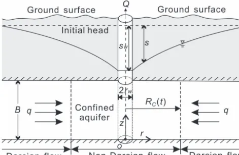
Figure 1. The schematic diagram of the non-Darcian flow into a fully penetrating pumping well considering the time-dependent crit-ical radius.
unique feature of the two-region model used in this study is that the critical radius is allowed to vary with time, whereas it was assumed to be constant in previous studies (Dudgeon et al., 1972b, a; Huyakorn and Dudgeon, 1976; Mackie, 1983; Sen, 1988; Wen et al., 2008b).
Generally, the start of the non-Darcian flow can be de-termined by the critical Reynolds number (ReC), where the Reynolds number is defined as
Re (r, t )=Dpq (r, t ) /ν, (1)
whereν is the kinematic viscosity of the fluid (L2T−1);Dp
is the characteristic grain diameter (L); q (r, t ) is specific discharge (LT−1) at distance r (L) and time t (T); Re is Reynolds number which depends on time and space (dimen-sionless). The critical Reynolds number (ReC)refers toRe at the start of non-Darcian flow. Up to present, there is still considerable debate onReCfor the initiation of non-Darcian flow in porous media. Scheidegger (1974) gave ReC to be 0.1 to 75; Zeng and Grigg (2006) suggested the range of
ReC from 1 to 100. ReC will be set to 100 to make sure non-Darcian flow happen in this study. According to Eq. (1), one can see that the specific discharge is in linear relation to Re. Therefore, the critical specific discharge (qC)can also be used to determine the start of the non-Darcian flow, since one can calculateqCfor a givenReC. When the specific dis-charge is less than or equal toqC(orRe≤ReC), the flow is considered as Darcian. When the specific discharge is greater than qC (or Re > ReC), the flow is taken as non-Darcian. Denoting RC(t ) as the critical radius at which q=qC (or Re=ReC), then it is non-Darcian flow whenr≤RC(t )and Darcian flow whenr > RC(t ), as shown in Fig. 1.
For the quasi steady-state flow around a fully penetrat-ing well in a homogeneous and isotropic formation, one has (Sen, 1988; Wen et al., 2008b)
RC=Q/ (2π BqC) , (2)
whereB is the thickness of the aquifer (L); and Q is the well discharge (L3T−1). In the case of a constant pumping rate,RCis also a constant for a specificReC. This constant RCwas used in previous two-region models of transient non-Darcian flow (Sen, 1988; Wen et al., 2008b). Actually,RCis not a constant for transient flow, and it cannot be determined directly since the velocity distribution changes with time. In this study, a new iteration method will be proposed to deter-mineRCas described below.
1.1.2 Mathematic model
Figure 1 shows the physical model investigated in this study, where a pumping well fully penetrates a confined aquifer. The origin of the cylindrical coordinate system is at the cen-ter of the well. Theraxis is horizontal and outward from the well, and thez axis is upward vertical. Three assumptions are made in this study. First, the non-Darcian and Darcian flow may coexist and the critical radius is time-dependent, and the non-Darcian flow is governed by the Forchheimer law. Second, the system is hydrostatic before the pumping starts, soRC(t=0)=0. Third, the aquifer is homogeneous, isotropic, infinitely extensive and with a constant thickness. These assumptions, although quite idealized, are standard in well hydraulic study (Papadopulos and Cooper, 1967; Sen, 1988; Wen et al., 2008b). Based on these assumptions, the governing equations of the two-region flow model can be de-scribed as follows
∂qN(r, t ) ∂r +
qN(r, t )
r =
S B
∂sN(r, t )
∂t , if r≤RC(t ) , (3) ∂qY(r, t )
∂r + qY(r, t )
r =
S B
∂sY(r, t )
∂t , if r > RC(t ) , (4)
wheresY(r, t )andsN(r, t )are drawdowns (L) at distancer and time t in Darcian flow and non-Darcian flow regions, respectively;Sis the aquifer storage coefficient (dimension-less).
Initial condition is
sY(r,0)=sN(r,0)=0. (5) The outer boundary condition is
sY(∞, t )=0. (6)
Assuming that the pumping rate is large enough to induce non-Darcian flow near the well, the boundary condition at the wellbore, considering the wellbore storage with a finite diameter well, can be written as
2π rBqN(r, t )
r→rw −π r 2 w
dsw(t )
dt = −Q, (7)
whereQis positive for the pumping rate;rwis the radius of the well (L);sw is the drawdown inside the well (L). Notice that well loss is not considered so the drawdown is continu-ous across the well screen
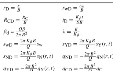
Table 1. Dimensionless variables used in this study.
rD=Br rwD=rBw RCD=RBC tD=KSBβt βd=2Qβπ B2 λ=KKβ
swD= 2π KQβBsw sYD=2π KQβBsY(r, t ) sND= 2π KQβBsN(r, t ) qND= −2π B
2
Q qN(r, t )
qYD= −2π B 2
Q qY(r, t ) qCD= −2π B 2
Q qC
The drawdown and the discharge from the Darcian flow re-gion into the non-Darcian flow rere-gion are continuous at the critical radius
sN[RC(t ) , t]=sY[RC(t ) , t], (9) qN[RC(t ) , t]=qY[RC(t ) , t]. (10) In the non-Darcian flow region, we use the Forchheimer law to describe the flow (Forchheimer, 1901)
qN+βqN|qN| =Kβ
∂sN
∂r , (11)
in which β (TL−1)andKβ (LT−1)are empirical constants
depending on the properties of the medium (Sidiropoulou et al., 2007).Kβ is called the apparent hydraulic
conductiv-ity and it reduces to the hydraulic conductivconductiv-ity whenβ=0 (Chen et al., 2001; Sidiropoulou et al., 2007).βis called the inertial force coefficient. Many studies demonstrated that the value ofβwas related to the porous media and the fluid prop-erties (Scheidegger, 1958; Moutsopoulos et al., 2009). For example, Ergun equation (Ergun, 1952) was widely used to estimateβ
β= 1.75Dp
150ν (1−ϕ), (12)
whereϕ is porosity. When the kinematic viscosity of water (ν)at 20◦C is 10−6m2s−1,Dp= 0.001 m,ϕ=0.3, one has
β=2.0×10⁻⁴m2day−1.
In the Darcian flow region, one has
qY(r, t )=K
∂sY(r, t )
∂r , r > Rc. (13)
Equations (3)–(13) can be used to describe the groundwa-ter flow in the aquifer with a time-dependent critical radius
RC(t ). This new model is an extension of the previous model by Sen (1988). WhenRC(t )→ ∞, this model becomes the F-ND model. When RC(t )=0, it reduces to the fully Dar-cian flow model.
1.1.3 Dimensionless transformation
Defining the dimensionless variables in Table 1, Eqs. (3)– (13) can be rewritten as
∂qND ∂rD
+qND
rD
= −∂sND
∂tD
, rD≤RCD, (14) ∂qYD
∂rD +qYD
rD
= −∂sYD
∂tD
, rD> RCD, (15) sND(rD,0)=sYD(rD,0)=0, (16)
sYD(∞, tD)=0, (17)
sND[RCD(tD) , tD]=sYD[RCD(tD) , tD], (18) qND[RCD(tD) , tD]=qYD[RCD(tD) , tD]. (19) Notice that a negative sign has been used for defining qD in Table 1. The subscript “D” stands for the dimensionless variables. The boundary condition with the wellbore storage (Eq. 7) in the dimensionless form is
(rDqND)
rD→rwD + rwD2
2S
dswD(tD) dtD
=1. (20) The dimensionless Forchheimer law becomes
qND+βDqND|qND| = − ∂sND
∂rD
, rD≤RCD, (21) where βD is the dimensionless inertial force coefficient. When the pumping rate is 0.628 m3s−1, aquifer thickness is 10 m, andβ=2.0×10⁻⁴m2day−1, one hasβ
D=0.02 ac-cording to the definition ofβD, as shown in Table 1.
WhenrD> RCD, groundwater flow follows the Darcy’s law in the dimensionless format as
qYD(r, t )= −λ ∂sYD
∂rD
, rD> RCD, (22) whereλis the ratio of the hydraulic conductivity and appar-ent (Sidiropoulou et al., 2007).
1.2 Numerical solution
Because of the non-linearity of the problem, it is not easy to obtain the analytical solution of drawdown even if
boundary (Mathias et al., 2008; Wen et al., 2009). For any node ofri,rwD< ri< reD,i=1, 2. . .N, one has
ri =(ri−1/2+ri+1/2)/2, i=1,2. . .N, (23) whereri+1/2is calculated as follows
log10(ri+1/2)=log10(rwD)+i log
10(reD)−log10(rwD) N
,
i=0,1. . .N. (24)
After spatial discretization, Eqs. (14)–(15) become dsYD,i
dtD
≈ri−1/2qYD,i−1/2−ri+1/2qYD,i+1/2
ri ri+1/2−ri−1/2
,
i=2,3. . .Ns−1, rD≤RCD, (25) dsND,i
dtD
≈ri−1/2qND,i−1/2−ri+1/2qND,i+1/2
ri ri+1/2−ri−1/2
,
i=Ns, Ns+1. . .N−1, rD> RCD, (26) where qYD,i and sYD,i are the dimensionless specific
dis-chargeqYD and dimensionless drawdownsYD at nodeifor the Darcian flow, respectively;qND,iandsND,iare the
dimen-sionless specific dischargeqNDand dimensionless drawdown sNDat nodeifor the non-Darcian flow, respectively. In terms of the Forchheimer equation of Eq. (21), one can obtain
qND,i−1/2≈ 1 2βD
( −1+
1+4βD
sND,i−1−sND,i
ri−ri−1
12) ,
i=2,3. . .Ns−1, (27)
and
qND,i+1/2≈ 1 2βD
( −1+
1+4βD
s
ND,i−sND,i+1 ri+1−ri
12) ,
i=2,3. . .Ns−1, (28)
where nodeNsmeans the location ofRCD(tD). At the well-aquifer boundary, one has
qND,1−1/2≈ 1 2βD
( −1+
1+4βD
swD−sND,1
r1−rwD 12)
, (29)
whereswD is the dimensionless drawdown inside the well. Considering Eq. (20),swDcan be approximated as follows
dswD dtD
≈ 2S
rwD2 1
−rwDqND,1−1/2. (30)
WhenrD> RCD, the finite-difference scheme of the specific discharge can be obtained from Eq. (22)
qYD,i−1/2≈λ
sYD,i−1−sYD,i
ri−ri−1
, i=Ns, Ns+1. . .N−1, (31)
qYD,i+1/2≈λ
sYD,i−sYD,i+1 ri+1−ri
, i=Ns, Ns+1. . .N−1. (32) As for the boundary at the infinity, the finite-difference scheme is
qYD,N+1/2≈λ sYD,N
reD−rN
. (33)
Now one obtains a set of ordinary differential equations. It is notable thatRCDorNs which is related to the indexiin Eqs. (27)–(28) and Eqs. (31)–(32) is time-dependent. In the following section, a new iteration method will be proposed to determine the values ofRCDorNs.
1.3 Iteration method to determineRCDorNs
Before introducing the new iteration method, the relationship betweenRCD and the velocity distribution will be investi-gated first, based on the two-region model with a constant
RCD. The values of the constantRCDare set to 0, 0.02, 0.04, 0.08 and 0.50. The other parameters are rwD=1×10⁻⁴, βD=20,λ=1. The mathematic model with a constantRCD will be solved by the finite-difference method.
Figure 2a shows the specific discharge distributions with different RCD of 0, 0.02, 0.04, 0.08 and 0.50. The curve of RCD=0 represents the fully Darcian flow model. One can find that the specific discharge decreases with increasing
RCD at a givenrD, starting from its maximum atRCD=0 (Darcian flow). This observation is understandable. The in-creasingRCDimplies a stronger contribution of the inertial effect, which also means a larger resistance to flow, thus it leads to a smaller specific discharge. After trying many dif-ferent sets of aquifer parameters, such asβD=0.002, 0.02, 0.2, and RCD=0.01, 0.03, 0.1, numerical simulation indi-cates that this observation is universally valid. This observa-tion will serve as the basis for the new iteraobserva-tion method to seek the location ofRCD(tD).
Similar to the use ofReCto determine the start of the non-Darcian flow, one can useqCDfor the initiation of the non-Darcian flow, whereqCDis the dimensionless critical specific discharge defined in Table 1. We denoterjCDas the newly computed critical radius at thejth step of the new iteration method, wherej=1,2,3. . .. Since the aquifer system is ini-tially hydrostatic, the initial critical radiusr0CD is set to 0. For a given dimensionless timet1D, the detailed procedures of the iteration method for searchingRCD(t1D)will be in-troduced as follows. First, the specific discharge distribution in the aquifer can be calculated using Eqs. (25)–(33) with
(a)
(b)
Figure 2. (a) Specific discharge distributions with different critical radiusRCD. (b) The schematic diagram showing the iterative pro-cess of seekingRCD.
lower limits for searchingRCD(t1D), as illustrated in Fig. 2b. Similarly, one can estimate the new critical radiusr3CDusing r2CD, wherer3CD is located somewhere between r1CD and r2CD. Following the same procedures, a new critical radius r4CD can be calculated based onr3CD, andr4CD is between r2CD andr3CD. One can repeat above computations until the new critical radius finally converges. For the actual problems, we define a convergence criterionRCDold−RnewCD
≤ξ, where RCDoldandRCDneware the critical radius for the previous step and present step, respectively; ξ is a small positive value such as 0.001. If this criterion is satisfied, the new critical radius
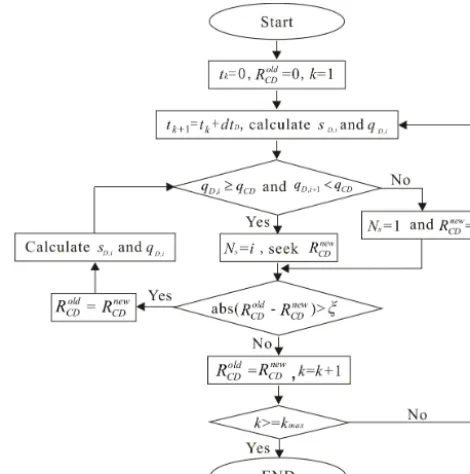
rjCDis thought as the estimation ofRCD(t1D). We develop a MATLAB program named as two-region model with moving critical radius (MTRM) to facilitate the computation. By the way, this iteration method is convergent. Figure 3 represents the flow chart of the MTRM algorithm, wheretk is the time
at time stepk;kmaxis the total number of the time steps; dtD is the dimensionless time step;sD,i andqD,i are the
[image:6.612.50.289.60.417.2]dimen-sionless specific drawdown and dimendimen-sionless discharge at nodeiin the aquifer, respectively.
Figure 3. Flow chart of the MTRM algorithm.
2 Results and discussions
2.1 Comparison with the previous solutions
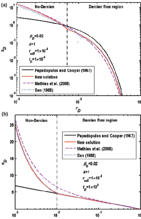
To test the new solution, the fully Darcian flow solution of Papadopoulos and Cooper (1967), the fully non-Darcian flow solution of Mathias et al. (2008) and the two-region model of Sen (1988) will be introduced. Figure 4a and b shows the distance-drawdown curves of the four mentioned-above models in the early and late pumping stages, respec-tively. In these two figures, Papadopoulos and Cooper (1967) represents the analytical solution of the fully Darcian flow model, Sen (1988) is the analytical solution of the two-region model by the Boltzmann transform method, and Mathias et al. (2008) represents the numerical solution of the fully non-Darcian flow model. The deflection point of the curve is the location of the critical radius.
[image:6.612.312.547.67.304.2](a)
(b)
Figure 4. (a) Comparison of the distance drawdowns by the fully Darcian flow model (Papadopoulos and Cooper, 1967), the fully non-Darcian flow model (Mathias et al., 2008), the two-region flow model (Sen, 1988), and the new model in early pumping stage. (b) Comparison of the distance drawdowns by the fully Darcian flow model (Papadopoulos and Cooper, 1967), the fully non-Darcian flow model (Mathias et al., 2008), the two-region flow model (Sen, 1988), and the new model in late pumping stage.
The fourth is that there is a deflection point on the new so-lution, leading to discontinuity of the drawdown slope. This observation may be reasonable, as also reported by Mout-sopoulos et al. (2009), who named it non-uniform hydraulic behavior.
[image:7.612.310.545.64.247.2]In the late pumping stage, the transient flow approaches the quasi steady state, and the specific discharge distribution is invariant with time according to Eqs. (3)–(4) or Eqs. (14)– (15), regardless of the Darcian flow or non-Darcian flow. Un-der the quasi steady-state flow condition, the critical radius obtained by this new solution becomes a constant which is the same as the one used by previous two-region models such as Sen (1988) and Wen et al. (2009). Therefore, the new so-lution agrees very well with that of Sen (1988) at late time
Figure 5. Time-dependent critical radius (RCD)for different values of the inertial force coefficientβD.
(see Fig. 4b). Another fact that can be seen in Fig. 4b is that the new solution agrees with the solution of Papadopoulos and Cooper (1967) in the Darcian flow region.
2.2 Effect of the inertial force coefficient to the critical radius
[image:7.612.50.287.66.433.2]The inertial force coefficient (βD) is of primary concern for the non-Darcian flow described by the Forchheimer equa-tion, and the values ofβDare chosen as 0.001, 0.01, and 0.1. Figure 5 shows the critical radius (RCD)changes with time for different dimensionless inertial force coefficients. Several observations can be seen. First,RCDincreases with time un-til the flow approaching the quasi steady-state condition. In the early pumping stage, the specific discharge is very large near the well and decreases quickly with the distance from the well, soRCD is very small. With time, the cone of de-pression will expand along the radial direction and the slope of the cone of depression becomes flatter, soRCD becomes greater. Second, a largerβDwould reduce the rate of change RCD versus time, thus result in longer time to approach its asymptotic value, and consequently leads to a smallerRCD at a specific time in the transient state (see Fig. 5). This is because a largerβD implies a stronger inertial force, which increases the resistance of flow. The third interesting obser-vation is that the asymptotic value ofRCD is the same for differentβD. This can be explained using Eq. (2). Based on the definition of the dimensionless parameters defined in Ta-ble 1, Eq. (2) becomes
qCD=1/RCD. (34)
Figure 6. Time-dependent critical radius (RCD)for different values of the critical specific discharge.
2.3 Effect of the critical specific discharge to the critical radius
The criterion to judge the initiation of the non-Darcian flow is an important factor of concern. Up to now, there is still considerable debate on what value ofReCto use for the start of non-Darcian low. The recommended values ofReCrange from 0.1 to 100 for porous media flow (Bear, 1972; Schei-degger, 1974; Zeng and Grigg, 2006). To check the influence of ReConRCDduring the transient flow, the values ofqCD are chosen as 100, 50 and 10 considering the direct relation-ship of qCD andRCD in Eq. (2). The other parameters are βD=0.01, andrwD=1×10⁻⁴.
Figure 6 shows the effect ofqCDonRCD. It is obvious that the asymptotic value ofRCDis equal to 1/qCD, as reflected in Eq. (34). Another interesting observation is thatRCD de-creases with increasingqCD, and it takes shorter time forRCD to approach its asymptotic value.
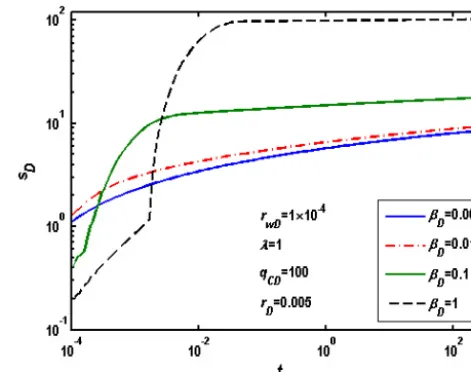
2.4 Type curves in the non-Darcian flow region and Darcian flow region
Type curves are a series of curves that reveal the functional relationship between the well functions (or drawdown) and the dimensionless time factors (Sen, 1988; Wen et al., 2011). Type curve is one of the common approaches to identify the aquifer parameters or to predict the drawdown (Sen, 1988; Wen et al., 2011). Sen (1988) presented different type curves in the Darcian flow region and non-Darcian flow region based on a two-region model. In that model (Sen, 1988),RCDwas a fixed value which only depends on the rate of pumping but independent of time. In this study,RCDchanges with time, and the type curves might be different from the ones gener-ated by Sen (1988). To investigate the behaviors of the type curves of the new solution, the two observation locations will
Figure 7. Time-drawdown atrD=0.005 for different inertial force coefficients in a log–log scale.
be chosen,rD=0.005 and 0.02. According to Eq. (34), the maximum ofRCD is 0.001 at the quasi steady state, so the flow atrD=0.005 will experience both Darcian flow (at the early time) and non-Darcian flow (at late time), while the flow atrD=0.02 is always Darcian.
Figure 7 shows the time drawdown atrD=0.005 for dif-ferent dimensionless inertial force coefficients in the log–log scale. Two interesting observations can be seen from this fig-ure. The first observation is that there is a deflection point in the curve ofβD=0.1 or 1, that becomes larger in time with increasingβD. This is because a largerβDimplies a stronger inertial effect, which leads to a larger drawdown and longer time to approach the quasi steady-state condition. This obser-vation is not found in the F-ND model (Wen et al., 2011) and in the two-region model (Sen, 1988). The second observation is that the drawdown in the quasi steady state increases with increasingβD, and the reason for this has been explained in previous studies (Wen et al., 2011).
Figure 8 represents the time drawdown atrD=0.02 in the log–log scale. One notable point is that flow atrD=0.02 is always Darcian, so there is no deflection point in the type curves. The differences among the curves with differentβD are obvious at the beginning, and then they approach the same value at the quasi steady state.
3 Summary and conclusions
[image:8.612.310.546.67.253.2]non-Figure 8. Time-drawdown atrD=0.02 for different inertial force coefficients in a log–log scale.
Darcian flow region, the flow is governed by the Forchheimer equation, and the start of the non-Darcian flow is determined by the critical specific discharge, which is calculated by the critical Reynolds number. The new solution is compared with previous solutions, such as the fully Darcian flow model, the two-region model with a constant critical radius, and the fully non-Darcian flow model. The impacts of the dimension-less inertial force coefficient (βD)and dimensionless critical specific discharge (qCD)on the critical radius and flow field have been analyzed. Several findings can be drawn from this study:
1. In the early stage, the new solution agrees with the fully non-Darcian flow solution near the well; differs with the fully Darcian flow model of Papadopoulos and Cooper (1967) and the two-region model of Sen (1988). 2. In the quasi steady flow stage, the new solution agrees with the solution of Sen (1988) very well. It agrees very well with the solution of the fully Darcian flow model (Papadopulos and Cooper, 1967) in the Darcian flow re-gion.
3. RCDincreases with time until reaching the quasi steady-state flow, and the asymptotic value of RCD only de-pends on qCD. A larger βD would reduce the rate of change ofRCDwith time, and result in a smallerRCD at a specific time during the transient flow state. 4. There is a deflection point in the type curve when the
[image:9.612.51.286.67.256.2]Appendix A
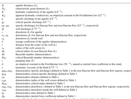
Table A1. Nomenclature.
B aquifer thickness (L)
Dp characteristic grain diameter (L)
K hydraulic conductivity of the aquifer (LT−1)
Kβ apparent hydraulic conductivity, an empirical constant in the Forchheimer law (LT−1)
q specific discharge in the aquifer (LT−1) qC critical specific discharge (LT−1)
qY,qN specific discharges for Darcian flow and non-Darcian flow (LT−1), respectively
Q well discharge (L3T−1) s drawdown (L) for aquifer
sY, sN drawdowns (L) for Darcian flow and non-Darcian flow, respectively
sw drawdown (L) inside well
S storage coefficient of the aquifer (dimensionless) r distance from the center of the well (L) rw radius of the well screen (L)
RC critical radius for non-Darcian flow (L) Re Reynolds number (dimensionless) ReC critical Reynolds number (dimensionless)
t pumping time (T)
β an empirical constant in the Forchheimer law (TL−1), named as inertial force coefficient in this study ν kinematic viscosity of the fluid (L2T−1)
qND, qYD dimensionless specific discharges defined in Table 1 in the non-Darcian flow and Darcian flow regions, respectively qCD dimensionless critical specific discharge defined in Table 1
rD dimensionless distance defined in Table 1
rwD dimensionless radius of the well screen defined in Table 1 RCD dimensionless critical radius defined in Table 1
sND, sYD dimensionless drawdownsdefined in Table 1 in the non-Darcian flow and Darcian flow regions, respectively
swD dimensionless drawdown inside the well defined in Table 1 tD dimensionless time defined in Table 1
βD dimensionless inertial force coefficient defined in Table 1
λ ratio of the hydraulic conductivity and apparent hydraulic conductivity defined in Table 1
Acknowledgements. This research was partially supported by
Program of the National Basic Research Program of China (973) (no. 2011CB710600, 2011CB710602), National Natural Science Foundation of China (no. 41172281, 41372253), the scholarship to Quanrong Wang from China Scholarship Council, Field Demonstration of Integrated Monitoring Program of Land and Resources in Middle Yangtze River Jianghan-Dongtin Plain (1212011120084), and Study on Groundwater Resources and En-vironmental Problems in Middle Yangtze River Jianghan-Dongtin Plain (no. 1212011121142). We thank two anonymous reviewers for the critical and constructive comments that help us improve this manuscript.
Edited by: S. Attinger
References
Ahmad, N.: Evaluation of groundwater resources in the upper mid-dle part of Chaj-Doak area, Pakistan, PhD, Istanbul Technical Univ., Turkey, 1998.
Basak, P.: Non-penetrating well in a semi-infinite medium with nonlinear flow, J. Hydrol., 33, 375–382, doi:10.1016/0022-1694(77)90047-6, 1977.
Basak, P.: Analytical solutions for two-regime well flow problems, J. Hydrol., 38, 147–159, 1978.
Bear, J.: Dynamics of fluids in porous media, Elsevier, New York, 1972.
Birpinar, M. and Sen, Z.: Forchheimer groundwater flow law type curves for leaky aquifers, J. Hydrol. Eng., 9, 51–59, doi:10.1061/(ASCE)1084-0699(2004)9:1(51), 2004.
Bordier, C. and Zimmer, D.: Drainage equations and non-Darcian modelling in coarse porous media or geosynthetic materials, J. Hydrol., 228, 174–187, doi:10.1016/s0022-1694(00)00151-7, 2000.
Camacho, R. G. and Vasquez, M.: Analytical solution incorporat-ing nonlinear radial flow in confined aquifers – comment, Water Resour. Res., 28, 3337–3338, doi:10.1029/92wr01646, 1992. Chen, Z. X., Lyons, S. L., and Qin, G.: Derivation of the
Forch-heimer law via homogenization, Transport in Porous Media, 44, 325–335, doi:10.1023/a:1010749114251, 2001.
Dudgeon, C. R., Huyakorn, P. S., and Swan, W. H. C.: Hydraulics of flow near wells in unconsolidated sediments, Field studies, The University of New South Wales, Australia, 1972a.
Dudgeon, C. R., Huyakorn, P. S., and Swan, W. H. C.: Hydraulics of flow near wells in unconsolidated sediments, Theoretical and experimental studies, The University of New South Wales, Aus-tralia, 1972b.
Dullien, F. A. L. and Azzam, M. I. S.: Flow rate pressure gradient measurements in periodically nonuniform capillary tubes, Aiche J., 19, 222–229, doi:10.1002/aic.690190204, 1973.
Engelund, F.: On the laminar and turbulent flows of ground water through homogeneous sand, Tech. Univ. Denmark, Copenhagen, Denmark, 1953.
Ergun, S.: Fluid flow through packed columns, Chem. Eng. Prog., 48, 89–94, 1952.
Forchheimer, P. H.: Wasserbewegung durch boden, Zeitsch-rift des Vereines Deutscher Ingenieure, 49, 1736–1749, 1901.
George, G. H. and Hansen, D.: Conversion between quadratic and power law for non-Darcy Flow, J. Hydraul. Eng.-ASCE, 118, 792–797, doi:10.1061/(asce)0733-9429(1992)118:5(792), 1992. Giorgi, T.: Derivation of the Forchheimer law via matched asymp-totic expansions, Transport in Porous Media, 29, 191–206, doi:10.1023/a:1006533931383, 1997.
Hassanizadeh, S. M. and Gray, W. G.: High-velocity flow in porous-media, Transport in Porous Media, 2, 521–531, 1987.
Huyakorn, P. and Dudgeon, C. R.: Investigation of 2-regime well flow, J. Hydraul. Division-ASCE, 102, 1149–1165, 1976. Irmay, S.: On the theoretical derivations of Darcy and Forchheimer
formulas – discussion – reply, J. Geophys. Res., 64, 486–487, doi:10.1029/JZ064i004p00486, 1959.
Izbash, S. V.: O filtracii V Kropnozernstom Materiale, Leningrad, USSR, 1931 (in Russian).
Liu, H. H., Li, L. C., and Birkholzer, J.: Unsaturated properties for non-Darcian water flow in clay, J. Hydrol., 430, 173–178, doi:10.1016/j.jhydrol.2012.02.017, 2012.
Louwyck, A., Vandenbohede, A., and Lebbe, L.: Numeri-cal analysis of step-drawdown tests: Parameter iden-tification and uncertainty, J. Hydrol., 380, 165–179, doi:10.1016/j.jhydrol.2009.10.034, 2010.
Mackie, C. D.: Determination of Nonlinear formation losses in pumping wells, International Conference on Groundwater and Man, 5–9 December, 1983.
Mathias, S. A. and Todman, L. C.: Step-drawdown tests and the Forchheimer equation, Water Resour. Res., 46, W07514, doi:10.1029/2009wr008635, 2010.
Mathias, S. A., Butler, A. P., and Zhan, H. B.: Approx-imate solutions for Forchheimer flow to a well, J. Hy-draul. Eng.-ASCE, 134, 1318–1325, doi:10.1061/(asce)0733-9429(2008)134:9(1318), 2008.
Mishra, P. K., Vessilinov, V., and Gupta, H.: On simulation and anal-ysis of variable-rate pumping tests, Ground Water, 51, 469–473, doi:10.1111/j.1745-6584.2012.00961.x, 2012.
Moutsopoulos, K. N., Papaspyros, I. N. E., and Tsihrintzis, V. A.: Experimental investigation of inertial flow pro-cesses in porous media, J. Hydrol., 374, 242–254, doi:10.1016/j.jhydrol.2009.06.015, 2009.
Papadopulos, I. S. and Cooper, H. H.: Drawdown in a well of large diameter, Water Resour. Res., 3, 241–244, doi:10.1029/WR003i001p00241, 1967.
Quinn, P. M., Parker, B. L., and Cherry, J. A.: Valida-tion of non-Darcian flow effects in slug tests conducted in fractured rock boreholes, J. Hydrol., 486, 505–518, doi:10.1016/j.jhydrol.2013.02.024, 2013.
Scheidegger, A. E.: The physics of flow through porous media, Uni-versity of Toronto Press, Toronto, 1974.
Scheidegger, A. E.: The physics of flow through porous media, Uni-versity of Toronto Press, 152–170, 1974.
Sen, Z.: Type curves for two-region well flow, J. Hydraul. Eng., 114, 1461–1484, doi:10.1029/WR024i004p00601, 1988.
Sen, Z.: Nonlinear radial flow in confined aquifers toward large-diameter wells, Water Resour. Res., 26, 1103–1109, doi:10.1029/WR026i005p01103, 1990.
Sidiropoulou, M. G., Moutsopoulos, K. N., and Tsihrintzis, V. A.: Determination of Forchheimer equation coefficients a and b, Hy-drol. Process., 21, 534–554, doi:10.1002/hyp.6264, 2007. Soni, J. P., Islam, N., and Basak, P.: A experimental evaluation
of non-Darcian flow in porous media, J. Hydrol., 38, 231–241, doi:10.1016/0022-1694(78)90070-7, 1978.
van Tonder, G. J., Botha, J. F., and van Bosch, J.: A generalised solution for step-drawdown tests including flow dimension and elasticity, Water S.A, 27, 345–354, 2001.
Ward, J. C.: Turbulent flow in porous media, J. Hydraul. Division, American Society of Civil Engineers, 90, 1–12, 1964.
Wen, Z., Huang, G. H., and Zhan, H. B.: An analytical so-lution for non-Darcian flow in a confined aquifer using the power law function, Adv. Water Resour., 31, 44–55, doi:10.1016/j.advwatres.2007.06.002, 2008a.
Wen, Z., Huang, G. H., Zhan, H. B., and Li, J.: Two-region non-Darcian flow toward a well in a confined aquifer, Adv. Wa-ter Resour., 31, 818–827, doi:10.1016/j.advwatres.2008.01.014, 2008b.
Wen, Z., Huang, G. H., and Zhan, H. B.: A numerical solu-tion for non-Darcian flow to a well in a confined aquifer using the power law function, J. Hydrol., 364, 99–106, doi:10.1016/j.jhydrol.2008.10.009, 2009.
Wen, Z., Huang, G. H., and Zhan, H. B.: Non-Darcian flow to a well in a leaky aquifer using the Forchheimer equation, Hydrogeol. J., 19, 563–572, doi:10.1007/s10040-011-0709-2, 2011.
Whitaker, S.: The Forchheimer equation: A theoretical development, Transport in Porous Media, 25, 27–61, doi:10.1007/bf00141261, 1996.
Yeh, H.-D. and Chang, Y.-C.: Recent advances in model-ing of well hydraulics, Adv. Water Resour., 51, 27–51, doi:10.1016/j.advwatres.2012.03.006, 2013.