FPGA Based Binary Heap Implementation: With an Application to Web Based Anomaly Prioritization

Georgia State University

ScholarWorks @ Georgia State University

Mathematics Theses Department of Mathematics and Statistics

12-16-2015

Numerical Solutions to Two-Dimensional

Integration Problems

Alexander Carstairs

Follow this and additional works at:https://scholarworks.gsu.edu/math_theses

This Thesis is brought to you for free and open access by the Department of Mathematics and Statistics at ScholarWorks @ Georgia State University. It has been accepted for inclusion in Mathematics Theses by an authorized administrator of ScholarWorks @ Georgia State University. For more information, please [email protected].

Recommended Citation

NUMERICAL SOLUTIONS TO TWO-DIMENSIONAL INTEGRATION PROBLEMS

by

Alexander D. Carstairs

Under the Direction of Valerie Miller, PhD

ABSTRACT

This paper presents numerical solutions to integration problems with bivariate integrands. Using

equally spaced nodes in Adaptive Simpson’s Rule as a base case, two ways of sampling the domain

over which the integration will take place are examined. Drawing from Ouellette and Fiume,

Voronoi sampling is used along both axes of integration and the corresponding points are used as

nodes in an unequally spaced degree two Newton-Cotes method. Then the domain of integration

is triangulated and used in the Triangular Prism Rules discussed by Limaye. Finally, both of these

techniques are tested by running simulations over heavily oscillatory and monomial (up to degree

five) functions over polygonal regions.

NUMERICAL SOLUTIONS TO TWO-DIMENSIONAL INTEGRATION PROBLEMS

by

Alexander D. Carstairs

A Thesis Submitted in Partial Fulfillment of the Requirements for the Degree of

Master of Science

in the College of Arts and Sciences

Georgia State University

Copyright by Alexander D. Carstairs

NUMERICAL SOLUTIONS TO TWO-DIMENSIONAL INTEGRATION PROBLEMS

by

Alexander D. Carstairs

Committee Chair:

Committee:

Valerie Miller

Rebecca Rizzo

Michael Stewart

Electronic Version Approved:

Office of Graduate Studies

College of Arts and Sciences

Georgia State University

ACKNOWLEDGMENTS

I would like to first thank my thesis advisor, Valerie Miller, for everything she has done to

help me complete this thesis. I would to also thank my committee members, Rebecca Rizzo and

Michael Stewart, for their feedback during the editing process. I am also grateful for all of my

classmates that have shared their wisdom and support throughout this process. Finally, I would

TABLE OF CONTENTS

ACKNOWLEDGMENTS . . . iv

LIST OF FIGURES . . . vii

LIST OF TABLES. . . viii

Chapter 1 INTRODUCTION . . . 1

1.1 Voronoi Sampling . . . 2

1.2 One-Dimensional Newton-Cotes Quadrature . . . 5

1.3 Delaunay Triangulation . . . 8

Chapter 2 ALGORITHMS . . . 12

2.1 Point Insertion Algorithms . . . 12

2.2 Incremental Delaunay Triangulation Algorithm with Edge Flips . . . 16

2.3 Complexity . . . 17

2.4 Delaunay Integration . . . 19

2.5 Monte Carlo Integration . . . 21

Chapter 3 IMPLEMENTATION AND NUMERICAL RESULTS . . . 25

3.1 Implementation . . . 25

3.2 Integrands . . . 27

3.3 Results . . . 28

Chapter 4 CONCLUSIONS AND FUTURE WORK . . . 39

Appendices . . . 42

Appendix A VORONOI SAMPLING MATLAB CODE . . . 43

Appendix B VORONOI NEWTON-COTES MATLAB CODE . . . 45

Appendix C DTRIS2 MATLAB CODE . . . 49

Appendix D BOWYER-WATSON ALGORITHM MATLAB CODE. . . 56

Appendix E RESULTS TABLES . . . 69

Appendix F SURFACE FIGURES . . . 74

LIST OF FIGURES

1.1 Descartes’ Diagram . . . 2

1.2 Delaunay Criterion . . . 3

1.3 2D Voronoi Diagram . . . 4

1.4 Voronoi Sampling . . . 4

1.5 Voronoi Diagram to Delaunay Triangulation . . . 9

1.6 Delaunay Criterion . . . 9

2.1 Bowyer-Watson Algorithm . . . 14

2.2 Edge Swapping . . . 16

2.3 Circumcircles and containment for triangulations of four points [13] . . . 18

LIST OF TABLES

1.1 Delaunay triangulation of 110 points . . . 11

2.1 Lawson’s algorithm. . . 13

3.1 Voronoi Newton-Cotes v. Adaptive Simpson’s Rule on Monomials Condensed . . . . 29

3.2 15000 Max Iteration of Voronoi Newton-Cotes v. Adaptive Simpson’s Rule . . . 30

3.3 Voronoi Newton-Cotes v. Adaptive Simpson’s Rule on Monomials Add. Pts. Con-densed . . . 31

3.4 Voronoi Newton-Cotes v. Adaptive Simpson’s Rule on Functions A-F . . . 31

3.5 Graphs of Functions A, B, C, D, E and F . . . 32

3.6 Condensed Simpson’s Cubature Rule v. Adaptive Simpson’s Rule on Monomials . . 33

3.7 Voronoi Newton-Cotes v. Adaptive Simpson’s Rule on Functions A-F . . . 34

3.8 Graphs of Functions A, B, C, D, E and F . . . 35

3.9 Condensed All Methods on Monomials Accuracy Only . . . 36

3.10 Condensed All Methods on Monomials Time Only . . . 37

3.11 All Methods on Functions A-F Accuracy Only . . . 37

3.12 All Methods on Functions A-F Time Only . . . 38

3.13 Graphs of Functions A, B, C, D, E and F . . . 38

E.1 Voronoi Newton-Cotes v. Adaptive Simpson’s Rule on Monomials . . . 69

E.2 Voronoi Newton-Cotes v. Adaptive Simpson’s Rule on Monomials Add. Pts . . . . 70

E.3 Simpson’s Cubature Rule v. Adaptive Simpson’s Rule on Monomials . . . 71

E.4 All Methods on Monomials Accuracy Only . . . 72

E.5 All Methods on Monomials Time Only . . . 73

F.1 Graphs of Monomial Functions . . . 74

Chapter 1

INTRODUCTION

The subject of numerical integration is an essential topic in any numerical analysis course, and

while there has been extensive research into numerical techniques, there is no unifying technique

that works for all integrands. Choosing a technique can be based on many factors, but ultimately

the decision will depend on the application. In the field of computer graphics, numerical integration

is essential in determining the lighting of an object. In [9], Fiume and Ouellette outline several

techniques for applications in computer graphics problems all of which must balance the numerical

efficiency of the method with the aesthetics of the final image, i.e. sacrificing numerical accuracy for

a better looking image. One of the methods outlined by Fiume and Ouellette is a one-dimensional

Voronoi diagram-based sampling of the domain of integration. In this thesis this sampling technique

will be expanded in two ways.

The first method is to perform the one-dimensional Voronoi sampling described in [9] along

each axis of integration to get two sets ofn points. Then the Cartesian product of those two sets

is taken to create an n×n grid of nodes, which can then be used in a quadrature method. The

second method will be to triangulate the domain of integration using a Delaunay triangulation.

These methods will be described in greater detail along with some relevant background theory of

each in Chapters 1 and 2, respectively. The Voronoi sampling will be implemented in an adaptive

Newton-Cotes method of degree two, and the Delaunay triangulation will be implemented in the

midpoint, trapezoidal and Simpson’s rules described in [3]. These methods, along with adaptive

Simpson’s rule and Monte Carlo integration, will be used to integrate a variety of test functions

described in [14] and the set of monomials given in [8]. The results of these numerical simulations

1.1 Voronoi Sampling

In this section, the reader is introduced to the basics of Voronoi diagrams. The following

definitions of the Voronoi diagrams are consistent with those given in [2] and [9]. The topic of

Voronoi diagrams dates back to the 1600s to Descartes where he used the idea that a set S of

sites(point sites)pin a space M are given and theregionof a site p consists of all pointss such

that the influence of p is the strongest. This concept emerged independently in various fields of

science such as biology to model and analyze plant competition; robotics to find an optimal path

to avoid a set of obstacles; and meteorology to determine regional rainfall from a discrete set of

rain gauges. In most of these cases, names particular to the field of study have been used, e.g.

Thiessen polygons are used in meteorology. The mathematicians Dirichlet and Voronoi would be

the first to formally introduce the concept while working with quadratic forms, and the resulting

structure has been given the name Dirichlet tessellation or Voronoi diagram [2].

Figure 1.1. Descartes’ diagram of the regions of influence for point sites [2]

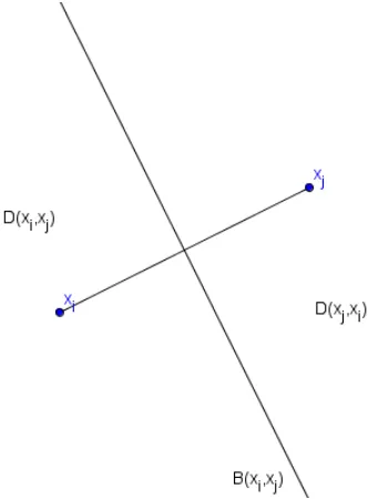
Definition 1.1.1. LetS ⊂_R2 _{be a set of points x}

1, x2, . . . , xn for n≥ 3 andp∈R2 with d(xi, p) given as some metric. For anyxi, xj ∈S and i6=j, let

be the bisector ofxi and xj, i.e. B(xi, xj) is the perpendicular line through the center of the line

segment connectingxi and xj. Thus, the bisector separates the halfplane

D(xi, xj) ={p|d(xi, p)< d(xj, p)}

containingxi from the halfplane D(xj, xi) containing xj.

Figure 1.2. Dividing halfplanes with bisector.

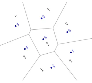
Using the halfplane described above, the Voronoi diagram can now be defined.

Definition 1.1.2. Let the Voronoi region of xi be given as

Vi =V(xi, S) =

\

xj∈S,i6=j

D(xi, xj)

with respect to S where Vi is an open set in the topological sense. Then the Voronoi Diagram of

S is defined as

V(S) = [

xi,xj∈S,i6=j

Vi∩Vj

whereV is the closure of set V, i.e. the open set V unioned with its boundary.

Figure 1.3. 2D Voronoi Diagram

a randomly chosen number from the uniform distribution over (a, b). Then the next n points are

determined by constructing the Voronoi regions corresponding to the location of the sample points

that already exist in the sequence. Let Vi represent the Voronoi region of xi and be defined as

Vi ={x∈[a, b]| |x−xj| ≤ |x−xi|, for all j ∈[1, n+ 3]}

for i ∈ [1, n + 3]. Let VM be the longest line segment as defined above with ties being broken

randomly. The next sample point in the sequence would the midpoint of the line segment

corre-sponding toVM. The abbreviationVmis used to denote a Voronoi sampling sequence ofnadditional

points wherem=n+ 3. In Fig 1.4, a quick example of the Voronoi sampling is given. Let a=−2,

b= 10 and x3 = 5. First, the midpoint (bisector) between the three points is found, which give us

m1 = 1.5 and m2 = 7.5. Then each Voronoi region is formed: V1 = (−2,1.5), V2 = (7.5,10) and

V3 = (1.5,7.5). Since V3 is the longest Voronoi region, the next point to be added to the sequence

isx4 = 4.5. The code written in MATLABc is given in Appendix A.

1.2 One-Dimensional Newton-Cotes Quadrature

Now it is necessary to derive a generic one-dimensional quadrature method for integrating

over [a, b]. Given three arbitrary points a, m and b, where a < m < b, Lagrange interpolation is

used to find a degree two polynomial to approximate our functionf(x). This polynomial is given

by

p(x) =

3

X

j=1

f(xj)Lj(x),

whereLj(x) is the Lagrange polynomial

Lj(x) =

3

Y

i=1,i6=j

x−xi

xj −xi

, j = 1,2,3

Thus,p(x) may be written as

p(x) =

3

X

j=1

f(xj)Lj(x) =f(a)

(x−m)(x−b)

(a−m)(a−b) +f(m)

(x−a)(x−b)

(m−a)(m−b)+f(b)

(x−a)(x−m) (b−m)(b−a) =τ

(1.2.1)

Assuming thatp(x) approximates some function f(x) that needs to be integrated then

Z b

a

f(x)dx≈ Z b

a

p(x)dx=

3

X

j=1

wjf(xj) =w1f(a) +w2f(m) +w3f(b),

where the weightswj are given by

wj =

Z b

a

Lj(x)dx.

All of these steps are similar to those for the derivation of an arbitrary Newton-Cotes method

using equally spaced points and are given in almost any numerical analysis textbook. Indeed, a

derivation of Simpson’s rule (sometimes referred to as Simpson’s 1/3 Rule) generally follows from

1.2.1 by exploiting the equal spacing of the points and gives a nice simplification.

Setting up a general spacing of points yields

b−m=α

a−m=−cα,

which simplifies the right hand side of Equation (1.2.1) to get

τ = 1

α2_{c(1 +c)}[f(a)(x−m)(x−b)−f(m)(1 +c)(x−a)(x−b) +cf(b)(x−a)(x−m)] (1.2.2)

To find the weights w1, w2 and w3 of f(a), f(m) and f(b), respectively, the function g(x) =

(x−u)(x−v) is integrated, which yields

Z b

a

(x−u)(x−v)dx= 1 2

(b−u)(b−v)2−(a−u)(a−v)2−1

6

(b−v)3 −(a−v)3=γ.

The right hand side of the above equation, γ, can then be simplified further according to the

following values ofu and v:

(i) If u=m, v=b: γ = 1₆α3_{(1 +c) (2c−1)}

(ii) If u=a, v=b: γ =−1 6α

3_{(1 +c)}3

(iii) Ifu=a, v=m: γ =−1 6α

3_{(1 +c)}2_(c−2)

Replacing the weights in (1.2.2) with the values above and simplifying gives

3

X

j=1

f(xi)Lj(x) =

α(1 +c) 6c

(2c−1)f(a) + (1 +c)2f(m) +c(2−c)f(b) .

This gives us our quadrature formula

I(f) =

Z b

a

f(x)dx≈ α(1 +c)

6c

(2c−1)f(a) + (1 +c)2f(m) +c(2−c)f(b) =I(p).

For the error, the equation

R(x) = I(f)−I(p) =

Z b _f000_(α)

is examined, and the function f is assumed to be at least three times differentiable over [a, b].

Since the cubic polynomial function changes sign over the interval [a, b], R(x) is broken into two

integrals in order to apply the weighted Mean-Value Theorem for Integrals:

R(x) = f

000_(α

1)

6

Z m

a

(x−a)(x−m)(x−b)dx+ f

000_(α

2)

6

Z b

m

(x−a)(x−m)(x−b)dx,

whereα1 ∈(a, m) and α2 ∈(m, b). It is now clear that only the general form of the integral above

is needed in order to proceed with the error analysis. Thus,

β =

Z v

u

(x−a)(x−m)(x−b)dx

= (v−u)

1

4(v+u)(v

2_+u2₎₋a+m+b

3 (v

2 _+uv+u2_{) +} am+ab+bm

2 (u+v)−amb

.

Simplifyingβ according to the following values of u and v:

(i) If u=a and v =m: β = (m−₁₂a)3 [2b−m−a]

(ii) If u=m and v =b: β = (b−₁₂m)3 [2a−m−b]

gives the total error R(x) to be

R(x) = f

000_(α

1)

6

(m−a)3

12 [2b−m−a] +

f000(α2)

6

(b−m)3

12 [2a−m−b]. (1.2.3)

Assuming thatf000 is essentially constant on [a, b], then

R(x)≈ A

6

(m−a)3

12 [2b−m−a] +

A

6

(b−m)3

12 [2a−m−b]

= A 72

(m−a)3[2b−m−a] + (b−m)3[2a−m−b]

= A

72(b−a)

3

[2m−b−a],

(b−m=α and a−m =−α) for the above error analysis, the same degree of accuracy for

Simp-son’s rule, but SimpSimp-son’s rule should have an extra degree of accuracy. The extra degree of accuracy

comes from the cancellation of the term containingf000 from the derivation of Simpson’s rule using

Taylor polynomials instead of Lagrange polynomials. To show this, Simpson’s rule is derived using

a Taylor expansion centered around the point m = b+₂a to approximate f(x). Integrating the

Taylor expansion from a tob to yields

Z b

a

f(x)dx=f(m)(b−a) + f

0_(m)

2

(b−m)2−(a−m)2+f

00_(m)

6 [(b−m)

3₋

(a−m)3]

+f

000_(m)

24

(b−m)4−(a−m)4

+ f

(4)_(ξ)

120

(b−m)5−(a−m)5

=f(m)(b−a) + f

0_(m)

2

(α)2−(−α)2+ f

00_(m)

6

(α)3−(−α)3+

f000(m) 24

(α)4−(−α)4+ f

(4)_(ξ)

120

(α)5−(−α)5

= 2αf(m) +α3f

00_(m)

3 +α

5f(4)(ξ)

60

= α

3[f(a) + 4f(m) +f(b)] +α

5f (4)_(ξ)

60 .

The f0 and f000 terms cancel, and the additional degree of accuracy is gained for Simpson’s rule.

The Voronoi sampling and quadrature are implemented in the functionvadapt3 and are given

in Appendix B.

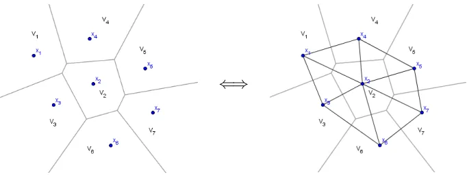
1.3 Delaunay Triangulation

According to Aurenhammer and Klein, Voronoi was the first to consider the dual of the

Voronoi diagram where he stated that any two point sites are connected if their regions share a

boundary. Later, Delaunay defined the dual in the following way:

Definition 1.3.1. Two point sites are connected if and only if the two sites lie on a circle whose

interior contains no point inS where S is the set defined in Definition1.1.1.

For this, the dual was given the name Delaunay tessellation or Delaunay triangulation. Given

a Voronoi diagram, one can easily construct a Delaunay triangulation by connecting the center

⇐⇒

Figure 1.5. Creating a Delaunay Triangulation from Voronoi diagram

it is not necessary to have a Voronoi diagram first. Using an alternate definition of a Delaunay

triangulation, a given triangulation can be checked to see if it is Delaunay.

Definition 1.3.2. A circumcircle is the circle that passes through the endpoints xi and xj for the

edge xixj and endpoints xi, xj and xk of triangle xixjxk for all combinations of i, j and k .

Definition 1.3.3. Let T be a triangulation with m triangles and a set of n points S where each

element ofS is a vertex of a triangleti ∈T for i= 1, . . . , m. T is consideredDelaunay if and only

if the circumcircle of every ti contains no other vertex in S.

Figure 1.6. Checking the Delaunay criterion holds for each triangle.

Both definitions 1.3.1 and 1.3.3 are known as the Delaunay criterion or empty circle

prop-erty for edges (1.3.1) and triangles (1.3.3), and are implemented in several algorithms used for

creating Delaunay triangulations. Since an edge only has two points, it can have infinitely many

circumcircles, but only one of the circumcircles has to be empty for the criterion to hold. On the

other hand, triangles will have a unique circumcircle defined by its three vertices, so there is only a

that it maximizes the minimum angle of all of the triangles within the triangulation of a given set

of points, which helps avoid skinny triangles. As the number of triangles increases, the triangles

appear more uniform in size as shown in Table 1.1. This reduces the risk of peaks on the function

that is being integrated from being cut off by large skinny triangles, which improves the stability

of the calculations performed on the mesh. In graphics, the uniformity of the triangles yields a

Chapter 2

ALGORITHMS

There are three types of algorithms used in the construction of Delaunay triangulations:

incremental insertion algorithms, divide-and-conquer techniques, and a sweepline techniques. The

simplest are the incremental insertion algorithms, and they can be expanded to be used in higher

dimensions. The algorithms that use the divide-and-conquer or sweepline techniques are faster

than the incremental insertion techniques in two dimensions but are difficult to generalize (if at

all) to higher dimensions. To construct the Delaunay triangulation in this thesis, two algorithms are

combined: the methoddtris2from the GEOMPACK package and the Bowyer-Watson algorithm.

Both algorithms are incremental insertion algorithms, which means they maintain a Delaunay

triangulation into which points are inserted [5]. First, dtris2 is used to triangulate the set of

initial points including the vertices along the boundary of integration and a randomly chosen

point within the boundary. The centroid of the largest triangle is then inserted using the

Bowyer-Watson algorithm. In the following sections, each algorithm is examined and shown how they are

implemented into our integration problem.

2.1 Point Insertion Algorithms

The earliest incremental insertion algorithm was developed by Lawson [11] and is based on

edge flips. When a vertex is inserted, the triangle that contains the new point is found, and the

point is connected to the vertices of the containing triangle by inserting three new edges. (If the

new point falls on the edge of an existing triangle, the edge is deleted, and the point is connected

to the four vertices of the containing quadrilateral by inserting four new edges). The edges are

placed into a stack and are tested to determine if they pass the Delaunay criterion. If not, then

added to the stack, and the algorithm ends when the stack is empty yielding a globally Delaunay

triangulation. A pictorial representation of Lawson’s algorithm is given below.

Table 2.1. Lawson’s algorithm.

In 1981 A. Bowyer and D. Watson simultaneously presented an algorithm that does not

depend on the use of edge flips and can easily be generalized to arbitrary dimensionality [11]. Our

implementation of the Bowyer-Watson algorithm is given below and starts

with already having a Delaunay triangulation of n points with a new point, xn+1, to be added.

1) Determine which triangle containsxn+1. Delete this triangle and add its neighbors to a stack.

2) Pop a triangle off the stack and determine if the new point is within the circumcircle of the triangle. If yes, delete the triangle and add the neighboring triangles to the stack.

3) Repeat 2 until stack is empty.

4) Triangulate the deleted region (The method dtris2 is used, which is discussed in the next section and our implementation is discussed in Chapter 3.).

Figure 2.1 shows the insertion of a point using the Bowyer-Watson algorithm. The Bowyer-Watson

algorithm can also be implemented from scratch with no preexisting triangulation. First, three

points are chosen that created a bounding triangle that encloses all of the points that need to

be triangulated. The algorithm as outlined above then follows. Once all of the points have

been inserted, the bounding triangle is then deleted along with all of its connections to the inner

triangulation.

Figure 2.1. Bowyer-Watson Algorithm: A: Circumscribing circles that contain the new point with the edges to be deleted ; B: resulting triangulation

As stated above, this algorithm easily generalizes to higher dimensions. When the new point

is inserted, the tetrahedron that contains the point is found, deleted and its neighbors are placed

into a stack. The tetrahedra in the stack are then checked to determine if their circumsphere is

empty. If the circumsphere is not empty, then the corresponding tetrahedron is deleted. Once the

stack is empty, the empty polyhedron that is left is “triangulated” and the process is repeated

until all points are inserted [11].

In its simplest form, this algorithm is not robust against roundoff error, though. A degenerate

case can develop in which two triangles have the same circumcircle, but only one of them is deleted

due to roundoff error, and the triangle that is not deleted is between the new vertex and the

triangle that was not deleted. This gives an empty cavity that is not empty, and the resulting

triangulation of the cavity would be“nonsensical” [11]. This problem can be avoided by using

Lawson’s algorithm instead. Lawson’s algorithm is not absolutely robust to roundoff error, but

Bowyer-Watson algorithm can be implemented with a depth-first search of the containing triangle

and will perform equally as robust as Lawson’s algorithm. Another advantage of Lawson’s is

that it is slightly easier to implement due in part because the topological structure maintained

throughout the process stays a triangulation [11]. The Bowyer-Watson was chosen due to the nice

pairing that it has with the method dtris2 below. The method keeps track of a neighbor matrix,

which virtually negates the search time for the triangles that are effected by the new insertion

point. The time complexity is discussed in further detail in Section 2.3.

There are many other methods that can be used for creating a Delaunay triangulation such

as divide-and-conquer approaches. The first O(nlogn) algorithm to create a Delaunay

triangula-tion was a divide-and-conquer approach that first created a Voronoi diagram then was dualized to

form the Delaunay triangulation. Due to the unnecessarily complicated process, another

divide-and-conquer approach was developed that directly constructed a Delaunay triangulation. In this

approach, the existing set of points are recursively divided into two groups, each group is

trian-gulated separately, and the groups are then merged together [7]. This algorithm proved to be as

intricate and cannot easily be implemented in higher dimensions. The approach proved to not be

as useful as Bowyer-Watson for our application for two reasons. First, this approach could have

been used instead of the Bowyer-Watson algorithm, but it would triangulate the entire set of points

after every point insertion as opposed to Bowyer-Watson, which only requires the triangulation of

a small subset after each point insertion. Secondly, the divide-and-conquer approach could have

been used in place of dtris2, but since dtris2 is only used for small subsets of triangles, there

was no added benefit to using the divide-and-conquer approach given its intricacy.

Another well-known approach is the sweepline method. This algorithm can also be

imple-mented in O(nlogn), and it builds a triangulation by sweeping a horizontal line vertically across

the plane with the triangulation accreting below the sweepline. When the sweepline collides with

a vertex, a new edge is created connecting the vertex to the sweepline. Once the sweepline reaches

the top of the circumcircle of a Delaunay triangle, the algorithm determines there is no other

vertex inside that circumcircle; thus, the triangle is created. This method also has restrictions

generalizing to higher dimensions and is not as easily implemented as the incremental insertion

methods. Similar to the divide-and-conquer approaches, the sweepline algorithm assumes that the

Figure 2.2. A: Edge e1 is not locally Delaunay since there is no empty circumcircle, perform edge

swap; B: e0 is locally Delaunay; C: the left triangle does not have an empty circumcircle, so not Delaunay, perform edge swap; D: both triangles have empty circumcircles, so both are locally Delaunay

[7],[11].

2.2 Incremental Delaunay Triangulation Algorithm with Edge Flips

The methoddtris2as described by Joe [5] is a variation of the algorithm given by Sloan [12].

Sloan’s algorithm combines the techniques from the Bowyer-Watson and Lawson algorithms. First,

a super triangle is created that encompasses all of the points to be triangulated. Then a point P

is inserted into the triangulation. The triangle that containsP is found, andP is connected to the

three vertices of the containing triangle to create three new triangles. The Lawson flip algorithm is

then used to make sure the triangulation is still Delaunay. This process is repeated until all points

have been inserted [12]. Joe uses the same outline for dtris2 but disregards the initial bounding

triangle and initially sorts the points lexicographically [5]. The algorithm in dtris2 is outlined

below by starting with a set of pointsS that needs to be triangulated.

1) Sort S using an ascending indexed heap sort to obtain the sorted set of indices Ss.

2) Take the first three points according to Ss and create the first triangle.

3) Add the next point according to Ss and connect the new vertex to the vertices that are

“visible” to the new point.

4) Check to make sure the new triangles are Delaunay. If not, perform edge swaps until all

The code for dtris2 translated into MATLABc is given in Appendix C. A crucial component

of this algorithm is that edge swapping guarantees the new triangles created are both Delaunay.

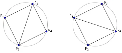
Welzl [13] provides the following proposition and proof that guarantees any four points that are

not cocircular have exactly one Delaunay triangulation.

Proposition 2.2.1. Given a set P ⊂_R2 _{of four points that are in convex position but not}

cocir-cular. Then P has exactly one Delaunay triangulation.

Proof. LetP =pqrs be a convex polygon (as shown in Figure 2.3). There are two triangulations

ofP: a triangulation T1 using the edgepr and a triangulationT2 using edge qs. Now consider the

family C1 of circles through the edge pr, which contains the circumcircles C1 =pqr and C10 =rsp

of the triangles in T1. By assumption s is not on C1. If s is outside of C1, then q is outside of C10.

Consider the process of continuously moving from C1 to C10 in C1 (left image in Figure 2.3) then

point q is “left behind” immediately when going beyond C1 and only the final circle C10 “grabs”

the point s.

Similarly, consider the family C2 of circles through pq, which contains the circumcircles C1 =

pqr and C2 = spq, the latter belonging to a triangle in T2. As s is outside of C1, it follows that

r is inside C2. Consider the process of continuously moving from C1 to C2 in C2 (right image in

Figure 2.3). The point r is on C1 and remains within the circle all the way up to C2. This shows

that T1 is Delauny, where as T2 is not.

The case that s is located inside C1 is symmetric; just cyclically shift the roles of pqrs to

qrsp.

2.3 Complexity

Now the time complexity of the dtris2 method and the Bowyer-Watson algorithm are

ana-lyzed. LetT be the time it takes to triangulate a set of n additional points be given as

T =

n

X

k=1

Tk+Sk, (2.3.1)

where Tk is the amount of time it takes to find the triangle that contains the new point and Sk

Figure 2.3. Circumcircles and containment for triangulations of four points [13]

in dtris2, Sk = O(1) because it is proportional to the number of triangles in the cavity not the

number of points. The reason for this is that the search for the neighboring triangle becomes

obsolete as the number of points in the triangulation increases. Experimentally, the number of

triangles in the cavity per iteration is less than ten, so as n increases the number of triangles

affected stays essentially constant; thus, making Tk the dominating factor. In the worst case the

complexity of Tk is O(k), which gives us O(n2) [1]. This worst case scenario happens when all

existing triangles’ circumcircles contain the new point at every point insertion. However, in the

typical case, the number of triangles to be deleted at each point insertion does not depend on the

number of existing triangles as described above. Combining anO(nlogn) multidimensional search

for the triangle that contains the new point and the saved information of the neighbor relations

between triangles, the Bowyer-Watson algorithm computes the Delaunay triangulation ofn points

inO(nlogn).

In [5], Joe discusses the time complexity of dtris2 and determines it to also be O(mlogm).

Since the method is only used for the initial set of points and the vertices along the hull of the cavity

along with the new point, then asnincreases,mstays relatively constant and is significantly smaller

than n. Thus, the time complexity of dtris2 and Bowyer-Watson together is stillO(nlogn).

Whenever implementing a geometric algorithm, two problems always need to be addressed:

geometric degeneracies and numerical errors. For the Delaunay triangulation, four or more

co-circular points will result in a non-unique triangulation [6] as shown in Figure 2.3. In such a

increasing order, triangle p1p2p3 will be created first. The point p4 will be added and triangle

p2p3p4 is created. It then checks to make sure that the triangulation is Delaunay, which it is,

so the method will move to the next point without considering the triangulation on the right.

Another geometric degeneracy that needs to be considered is if three or more points are too close

to being co-linear. In this case,dtris2 checks for a “healthy” triangle when inserting a new point.

It determines this by checking if the third point is to the left or right of a directed ray between

the initial two points of the triangle. If the third point is within a certain tolerance of the directed

ray, the method will break and return a fatal error.

Figure 2.4. Two valid Delaunay triangulations with four co-circular points.

Numerical errors are more difficult to handle. As discussed in Section 2.1, there is a degenerate

case for roundoff error in the Bowyer-Watson algorithm. Mavriplis also discusses this issue with

round-off error in [7]. In general, the nature of the problem will determine the accuracy

require-ments of the inputs and outputs. For our implementation, double-precision arithmetic is used, and

it proves to be very robust. An occasional error occurs when inserting several thousand points in

dtris2 that appears to happen when two points are too close to each other, which illustrates the

round-off error problems described in Section 2.1. Since the error rarely occurred, the iteration

was simply skipped but noted during the simulation process using a try/catch block.

2.4 Delaunay Integration

Now the triangulation of the integral domain is implemented in the triangular prism rules

described in [3] to approximate the integral

Z Z

D

function f(x, y) above with a two variable polynomial function p2 of total degree 2 whose values

at the points (x1, y1), (x2, y2), and (x3, y3) and (x1+₂x2,y1+₂y2), (x2+₂x3,y3+₂y3), and (x3+₂x1,y3+₂y1) are

equal to the values at f(x, y) at the same points. Then the “signed volume” under the surface

given byp2(x, y) is the “volume” of the paraboloidal triangular prism with its base Di, the lengths

of the 3 parallel edges equal to f(x1, y1), f(x2, y2), f(x3, y3), and the heights at the midpoints of

the sides are equal to the values of f(x, y) at those midpoints. This gives us a “cubature”[3] rule

in two variables that is analogous to Simpson’s rule in one-variable and is given by

Z Z

Di

f(x, y)dxdy≈ Area(Di)

3

f(x1+x2 2 ,

y1 +y2

2 ) +f(

x2+x3

2 ,

y2+y3

2 ) +f(

x3+x1

2 ,

y3+y1

2 )

,

(2.4.2)

whereDi ∈Dfor alli= 1,2, . . . , n. Although the 2D Simpson’s rule is the main method in which

our triangulation is implemented, the midpoint and trapezoidal equivalents described in [3] are

also used for added performance comparison.

For the midpoint rule, let (s, t) be the centroid of Di and replace the function f(x, y) from

2.4.1 with the constant functionp0(s, t). The “signed volume” under the surface given byp0 is the

“volume” of the triangular prism with the base Di and height f(s, t). This gives the “cubature”

rule as

Z Z

Di

f(x, y)dxdy≈Area(Di)f(s, t) =Area(Di)f

x1+x2+x3

3 ,

y1+y2+y3

3

,

where Di ∈D for all i= 1,2, . . . , n. Now replace the functionf(x, y) in 2.4.1 with a two variable

polynomial function p1 of total degree 1 whose value at (xi, yi) is equal to f(xi, yi) for i = 1,2,3.

The “signed volume” under the surface given by p1(x, y) is the “volume” of the obliquely cut

triangular prism with base Di, and the length of the three parallel edges are f(x1, y1), f(x2, y2)

and f(x3, y3). This gives us the two variable trapezoidal rule defined by

Z Z

Di

f(x, y)dxdy ≈Area(Di) [f(x1, y1) +f(x2, y2) +f(x3, y3)],

2.5 Monte Carlo Integration

Monte Carlo methods are numerical methods that depend on taking random samples to

ap-proximate their results. Monte Carlo integration applies this process to the numerical estimation

of integrals. In this section some of the fundamental properties of Monte Carlo integration as

de-scribed by Jarosz are given. All of the definitions and descriptions below are consistent with those

found in [4] but can be found in most sources that discuss probability and Monte Carlo methods.

Suppose random variableX, then thecumulative distribution function, or CDF, ofXis defined

as

cdf(x) = P {X ≤x} (2.5.1)

The corresponding probability density function, or PDF, is defined as the derivative of CDF, i.e.

pdf(x) = d

dxcdf(x). (2.5.2)

From 2.5.1 and 2.5.2, an important relationship forms that allows us to determine the probability

that a random variable lies between two values:

P {a≤x≤b}=

Z b

a

pdf(x)dx.

Now the expected values and variance of a random variable are investigated. Consider the

random variable Y =f(x) over a domain µ(x) then the expected value is defined as

E[Y] =

Z

µ(x)

f(x)pdf(x)dx, (2.5.3)

and thevariance is defined as

σ2[Y] =E(Y −E[Y])2, (2.5.4)

where σ is the standard deviation and is the square root of the variance. From 2.5.3 and 2.5.4, it

E[aY] =aE[Y], (2.5.5)

σ2[aY] =a2σ2[Y].

Furthermore, the expected value of the sum of random variables Yi is equal to the sum of their

expected values:

E "

X

i

Yi

#

=X i

E[Yi]. (2.5.6)

Combining these properties, 2.5.4 simplifies to the following:

σ2[Y] =EY2−E[Y]2.

Now, suppose f(x) is to be integrated over [a, b]:

F =

Z b

a

f(x)dx.

The integral, F, can then be approximated by averaging samples of the function f at random

points from a uniform distribution between a and b. Given a set of n uniform random variables

Xi ∈[a, b) with corresponding PDF of _b−1a, then the Monte Carlo estimator for F is

hFni= (b−a) 1

n−1

n

X

i=0

f(Xi). (2.5.7)

SincehFn_{iis a function of X}

i, then it is a random variable as well, and this notation will be used

to denote that hFni is an approximation of F using n samples. Intuitively, equation 2.5.7 can be

viewed two ways: 1) the estimator in 2.5.7 computes the mean value of the functionf(x) over [a, b]

and multiplies by length of the interval (b−a), or 2) by moving (b −a) inside the summation,

the estimator is choosing the height at a random evaluation of the function and averaging a set of

rectangular areas computed by multiplying this height by the length of the interval (b−a). It is

E[hFni] =E "

(b−a)1

n

n−1

X

i=0

f(Xi)

#

= (b−a)1

n

n−1

X

i=0

E[f(Xi)] from eqns. 2.5.5 and 2.5.6

= (b−a)1

n

n−1

X

i=0

Z b

a

f(x)pdf(x)dx from eqn. 2.5.3

= 1

n

n−1

X

i=0

Z b

a

f(x)dx since pdf(x) = 1

b−a

=

Z b

a

f(x)dx

=F.

As n increases, the estimator hFn_{i becomes closer to F, and due to the Strong Law of Large}

Numbers, the exact solution is guaranteed in the limit:

P nlim

n→∞hF

n_i=Fo_{= 1.}

For the one-dimensional case, the convergence rate is determined by looking at the convergence

rate of the estimator’s variance:

σ[hFni]∝ √1 n.

Even though the convergence rate is slow compared to other one-dimensional techniques, it does

not get exponentially worse like many other techniques as the dimension increases. For instance,

a deterministic quadrature requires using nd _{samples for a d-dimensional integral, but the Monte}

Carlo techniques provide the ability to choose any arbitrary number of points. The estimator,hFn_i,

can easily be extended to multiple dimensions by using random variables drawn from arbitrary

PDFs and solving the following:

F =

Z

ω

f(¯x)dx,¯

hFni= 1

n

n−1

X

i=0

f(Xi)

pdf(Xi)

.

Similar to before when showing E[hF2_{i] = F for pdf(x) =} 1

b−a, the extended estimator has the

correct expected value:

E[hFni] =E "

1

n

n−1

X

i=0

f(Xi)

pdf(Xi)

# = 1 n n X i=0 E

f(Xi)

pdf(Xi)

= 1

n

n−1

X

i=0

Z

ω

f(¯x)

pdf(¯x)pdf(¯x)dx¯

= 1

n

n−1

X

i=0

Z

ω

f(¯x)dx¯

=

Z

ω

f(¯x)dx¯

=F.

As mentioned above the convergence rate stays constant atO(√1

n) with the added dimensions, so

σ[hFni]∝ √1 n.

The convergence rate can be improved by a variety of techniques that mainly deal with reducing

the variance using more advanced sampling techniques, but for our purposes, the convergence rate

atO(√1

Chapter 3

IMPLEMENTATION AND NUMERICAL RESULTS

In this chapter the implementation of the algorithms and theory that was presented in the

previous chapters is given. Then test functions are defined, and the numerical results given by

testing our implementations versus other known techniques discussed in Chapter 2 are also

dis-cussed. First, the adaptive Newton-Cotes quadrature discussed in Section 1.2 is tested against

adaptive Simpson’s. Then adaptive Simpson’s is compared to Simpson’s rule over the Delaunay

triangulation described in equation (2.4.2). Finally, the performance of all of the techniques are

compared to each other simultaneously.

3.1 Implementation

In Sections 2.1 and 2.2, the Bowyer-Watson algorithm and the method dtris2 were

inves-tigated. These methods were combined to create a hybrid method that is based mainly on the

Bowyer-Watson algorithm. Starting with an array,P, that contains the four points representing the

vertices of the rectangular integration domain and one randomly chosen point within the rectangle,

the initial triangulation is constructed using the dtris2 method. From this initial triangulation,

dtris2 produces three outputs: the number of triangles, a matrix verts that gives the vertices

of each triangle and another matrix nabes that gives the neighbor relations of the triangles. The

columns of each matrix refers to a triangle in the triangulation, i.e. column one refers to triangle

T1, column two refers to triangle T2, etc. The values of verts are indices referencing the location

(>0) or a boundary edge (<0). For example, let verts=     

2 5 5 2

1 1 3 5

5 3 4 4

     and nabes=     

−7 1 2 1

2 −10 −14 3

4 3 4 −3



   

thenT1 has vertices visited counterclockwiseP2, P1 and P5, andT1 also neighbors trianglesT2 and

T4 along the edges P1P5 and P5P2 with edge P2P1 being a boundary edge.

Then the affected region is found by determining which triangles’ circumcircles contain the

new point. The boundary of the affected region is then stored in a temporary matrix with the

newly inserted point. The region is then triangulated using dtris2. If the region is concave then

the triangles that are created from bridging the concave vertices are deleted. If the region is convex

then the triangulation is correct, and there is no need to delete any triangles.

Now that the affected region is triangulated, it needs to inserted back into the main

trian-gulation. To do this, the referencing between the neighbor and vertex matrices of the affected

region need to be inserted into the neighbor and vertex matrix for the main triangulation. First

the point references in the vertex matrix are corrected. When triangulating the affected region

with m points, dtris2 labels the points 1,2, . . . , m, so the references need to be changed to their

original numbering from P that consists ofn points. Similar to the vertex matrix for the affected

region, the neighbor matrix is also updated to reflect the numbering of the whole triangulation.

While correcting the numbering of nabes, the entries that are boundary edges for the affected

region are set to 0 if they are not a boundary edge for the entire triangulation. If they are a

boundary edge for both the affected region and larger triangulation, then the entry remains the

same. Then the vertex and neighbor matrices for the affected region are merged with verts and

nabescorresponding to the overall triangulation. This is done by first noticing that if m triangles

were affected, then the new triangulation consists of m+ 2 triangles, so each column in nabes

onto the end. The corresponding columns in the vertex matrix for the affected region are added

in the same manner toverts. The vertex matrix is now complete and describes the triangulation

with the new point added. Lastly, all of the zeros in nabes are changed to their correct triangle

references, and all of the negative entries are updated as well. The triangulation is now complete

with correct vertex and neighbor matrices,verts and nabes, respectively. The code can be found

in Appendix D.

The algorithm described above is used in the cubature rules described in Section 2.4. The

implementation of each of the cubature rules follows the same general outline with the only

differ-ence being at what points the function is being evaluated as given by each rule. First, an initial

triangulation is found usingdtris2 along with the areas of each triangle. The areas are then placed

array in increasing order, and a matrix containing the boundary edge information is also created.

Then the functions is “integrated” using one of the three cubature rules described in [3] (Simpson’s,

midpoint and trapezoid). The error is then calculated to see if it is within the given tolerance.

If the volume is not within the given tolerance then the triangle with largest area is selected for

refinement, and its centroid is computed. This point becomes the new point to be inserted and

the algorithm above is run to determine the new triangulation. After triangulating, the areas of

the triangles affected during the triangulation are deleted, and the new ones are calculated and

sorted in ascending order. The two arrays of areas are then merged together. This process repeats

until the volume is within the given tolerance or a maximum number of iterations is reached.

This method involving the cubature rules is not implemented adaptively, so the error at each step

is compared to the previous step. However, the Voronoi Newton-Cotes method is implemented

adaptively similar to our base case of the two-dimensional adaptive Simpson’s Rule.

3.2 Integrands

In [14], Yu and Sheu examine solving the following double integral using the Mean-Value

theorem for integrals:

Z 2π

0

Z R

0

wheres, φ, R∈_R, R >0, n∈_Z+ _{and f(r, θ, s, φ, n) is one of the following functions:}

A(r, θ, s, φ, n) = rexp

" _n X k=0 n k

sn−krkcos [(n−k)φ+kθ]

# cos " _n X k=0 n k

sn−krksin [(n−k)φ+kθ]

#

,

(3.2.1)

B(r, θ, s, φ, n) =rexp

" _n X k=0 n k

sn−krkcos [(n−k)φ+kθ]

# sin " _n X k=0 n k

sn−krksin [(n−k)φ+kθ]

#

,

(3.2.2)

C(r, θ, s, φ, n) = rsin

" _n X k=0 n k

sn−krkcos [(n−k)φ+kθ]

# cosh " _n X k=0 n k

sn−krksin [(n−k)φ+kθ]

#

,

(3.2.3)

D(r, θ, s, φ, n) = rcos

" _n X k=0 n k

sn−krkcos [(n−k)φ+kθ]

# sinh " _n X k=0 n k

sn−krksin [(n−k)φ+kθ]

#

,

(3.2.4)

E(r, θ, s, φ, n) = rcos

" _n X k=0 n k

sn−krkcos [(n−k)φ+kθ]

# cosh " _n X k=0 n k

sn−krksin [(n−k)φ+kθ]

#

,

(3.2.5)

F(r, θ, s, φ, n) = rsin

" _n X k=0 n k

sn−krkcos [(n−k)φ+kθ]

# sinh " _n X k=0 n k

sn−krksin [(n−k)φ+kθ]

#

.

(3.2.6)

Even though n can be an any integer such that n ≥ 1, it is only chosen to be between 1 and 3.

Whenn is increased, the results would become quite large (≥106_{) most of the time, which made it}

more difficult to get a good graph and harder to determine what could be causing the inaccuracies.

The methods were also tested on functions of the form

Z d

c

Z b

a

xiyjdxdy

wherea, b, c, d∈_R, i, j ∈_Z+ _{and i+j ≤5.}

Analytical solutions for eachf(r, θ, s, φ, n) is provided by Yu and Sheu, so the relative errors

of each trial could easily be calculated. Similarly, the analytical solutions for the monomials can

be found, so the relative error could easily be calculated.

3.3 Results

The Voronoi Newton-Cotes method is initially tested against Simpson’s rule on the set of

additional points between our boundaries at each step similar to how Simpson’s rule finds the

three midpoints (quartiles) between the boundaries. For all of the simulations shown in the

ta-ble, a tolerance of = 0.0001 is used, and the function is integrated over four randomly chosen

points to create a rectangle with vertices a = −0.00884120840760527, b = 2.71855632151155, c

= 2.88900981641759, d = 3.44868288240732. The full results of one of the simulations are given

in Table E.1 in Appendix E, and the graphs of the functions are given in Table F.1 in Appendix

F. From Table 3.1, it is obvious that the Voronoi Newton-Cotes Method is exact (within machine

epsilon) for polynomials of degree two or less but is not always exact for the polynomials of degree

three. As given in Equation 1.2.3, this is expected since the interpolating polynomial is only exact

through degree two, and there is no additional degrees of accuracy since the error term is only

proportional tof(3)_{. Also, it is clear that Simpson’s rule is exact through degree three as expected}

as illustrated in Table 3.1.

Table 3.1. Condensed Voronoi Newton-Cotes (VNC) v. Adaptive Simpson’s Rule (AS) on Monomials with a = −0.00884120840760527, b = 2.71855632151155, c = 2.88900981641759, d = 3.44868288240732 and = 0.0001.

i j AS Time AS Rel. Error VNC Time VNC Rel. Error 0 0 0.008355225 1.45465E-16 0.007077289 0

0 1 0.000445179 1.83618E-16 0.000605689 1.83618E-16 0 2 0.000444923 1.15589E-16 0.000636664 1.15589E-16 0 3 0.000717303 1.45154E-16 0.028169894 4.20143E-08

1 0 0.00050585 0 0.000657144 0

1 1 0.000572153 1.35526E-16 0.000752119 2.71052E-16 1 2 0.000714487 3.41259E-16 0.000930037 3.41259E-16 2 0 0.000655608 1.18479E-16 0.000882165 1.18479E-16 2 1 0.000450042 4.48665E-16 0.000632312 1.49555E-16 3 0 0.000457722 1.16218E-16 0.498908685 8.96198E-08

For the higher degree (≥ 4) polynomials shown in Table E.1 in Appendix E, the Voronoi

Newton-Cotes method performs adequately giving four additional orders of accuracy for the given

epsilon in many cases. However, there are three cases that notably stand out: f(x, y) = x3_y2_,

f(x, y) = x4y1 andf(x, y) = x5, which are examined further in Table 3.2. Originally the maximum

number of iterations was set to 5000, and all three of those cases reached the maximum number,

are shown in Table 3.2. The relative errors again give us an additional four or five digits of accuracy

Table 3.2. 15000 Max Iteration Voronoi Newton-Cotes (VNC) v. Adaptive Simpson’s Rule (AS) on Monomials with a = −0.00884120840760527, b = 2.71855632151155, c= 2.88900981641759, d

= 3.44868288240732 and = 0.0001.

i j AS Time AS Rel. Error VNC Time VNC Rel. Error Iterations

3 2 0.000457210 0 3.063991277 1.30530E-08 6497

4 1 0.116197996 4.03868E-08 4.288516134 2.32547E-09 9069 5 0 0.211611352 7.10947E-08 7.329204530 3.50050E-08 14869

and even outperform adaptive Simpson’s rule on one of the runs. Unfortunately, the amount of

time taken spiked drastically. Since the desired accuracy was finally achieved, the next step was

to try to improve the speed of the method.

As stated above, the trials were initially run using the adaptive Voronoi Newton-Cotes with

the Voronoi sampling only being used for three additional points along each axis. When examining

the intermediate steps of both methods, the Voronoi Newton-Cotes had very long streaks of not

adding any values to the total volume. This meant it was spending a lot of time finding an accurate

enough approximation to be able to move on to the next quadrant. When looking at how the points

were generally distributed between the two values, there were large gaps on the tails of the interval

giving large areas to approximate over on the ends, which would then need more refinement. Since

Simpson’s rule uses the midpoints of each cell at every step, the empty space is filled much more

evenly than with the Voronoi sampling; therefore, Simpson’s rule was always using significantly

fewer iterations. In an effort to correct this, more points were sampled at each step (19 additional

for a total of 21 with the endpoints) but would only use the first, second and third quartiles of

the sampling. As shown in Table 3.3, the guaranteed accuracy through degree two for Voronoi

Newton-Cotes and degree three for Simpson’s rule remains unchanged. In Table E.2, the times for

the larger degree polynomials and did end up improving with the accuracy remaining roughly the

same as before. Since increasing the number of points helped the speed of the algorithm and also

gave us similar accuracy, the Voronoi sampling of 19 points over the three point method is used inn

the rest of the trials described in this thesis. Even with the additional increase in speed, adaptive

Simpson’s provides both better accuracy and speed on these simple functions overall, though. Now

Table 3.3. Condensed Voronoi Newton-Cotes (VNC) v. Adaptive Simpson’s Rule (AS) on Monomials with additional sampling anda = −0.00884120840760527, b = 2.71855632151155, c= 2.88900981641759, d = 3.44868288240732 and = 0.0001.

i j AS Time AS Rel. Error VNC Time VNC Rel. Error 0 0 0.001667055 0 0.005648840 1.45465E-16 0 1 0.000532987 0 0.001388274 3.67237E-16 0 2 0.000424188 2.31179E-16 0.001337843 0 0 3 0.000500475 1.45154E-16 0.022388000 4.90503E-08 1 0 0.000477947 0 0.001335283 4.29461E-16 1 1 0.000468731 1.35526E-16 0.001387250 0 1 2 0.000577018 0 0.001409522 1.70629E-16 2 0 0.000573178 2.36958E-16 0.001332467 4.73917E-16 2 1 0.000468475 2.99110E-16 0.001327091 1.49555E-16 3 0 0.000555770 1.16218E-16 0.432514594 4.00847E-08

Next tests were run on the functions described above from [14] using Voronoi Newton-Cotes

and Simpson’s rule. For all of the simulations shown in Table 3.4, again a tolerance of= 0.0001

is used, and the function is integrated over the rectangle given bya = 0, R = 5.480255137, c= 0,

d = 2π with R being a randomly chosen point. The parameters s, φ and n are randomly chosen

to bes= 2.444171059,φ = 5.69125859039527 and n= 1.

Table 3.4. Voronoi Newton-Cotes (VNC) v. Adaptive Simpson’s Rule (AS) on Functions A-F with a = 0, R = 5.480255137, c= 0, d = 2π, s= 2.444171059, φ = 5.69125859039527, n = 1 and

= 0.0001.

f

Type AS Time AS Rel. Error VNC Time VNC Rel. Error A 11.8374406 2.729767377 16.11166813 1.182096082 B 12.04885046 1.418534859 16.38065796 0.842777814 C 12.13505427 1.611736343 16.61918614 1.067504856 D 13.03777242 2.358085297 17.13948942 0.634025761 E 12.37735201 2.191400672 18.07931543 0.806867337 F 12.78167719 1.697312935 17.24927674 0.899201229

It is clear to see from Table 3.4 that neither Simpson’s rule nor the Voronoi Newton-Cotes

method performs well on the six functions. Looking at the graphs of these functions in Table

3.5, these functions have fairly sharp high and low peaks and are also oscillatory. Simpson’s rule

functions appear to have equally high and low peaks, a similar cancellation could be affecting the

results. It is easy to see that the Voronoi Newton-Cotes method could also run into a similar

problem given the right function and “midpoint.”

Table 3.5. Graphs of Functions A-F with a= 0, R = 5.480255137, c= 0, d= 2π,

s= 2.444171059, φ= 5.69125859039527,n = 1 and = 0.0001.

Similar to our simulations comparing the methods on monomials, the results displayed in

Table 3.4 have a maximum number of iterations of 5000. As before, the maximum number of

iterations was increased, this time all the way to 20000, but this did not improve the accuracy by a

significant amount (rarely getting even one additional order of accuracy). Ignoring the accuracy and

looking at the times it took to complete the simulation, Simpson’s rule still trumps the

Newton-Cotes method. Since both of the simulations are now executing the same number of iterations

(5000), it is highly likely the time difference is attributed to the extra work the Voronoi

Newton-Cotes has to do to perform the extra sampling.

Now that the Voronoi Newton-Cotes method and Simpson’s rule have been compared against

each other, Simpson’s rule is now compared against the Simpson’s rule analog using the

the performances of Simpson’s rule and Simpson’s cubature rule will first be compared over the

monomials to make sure the expected guaranteed accuracies hold. Then they will be tested on

the higher degree monomials. Both methods use a tolerance of = 0.0001 over the rectangle a

=−1.62110966800282,b =−1.37432067059289,c= −3.3239379751915,d = −1.72003265166653.

The results for the entire simulation are given in Table E.3 in Appendix E. Looking at Table 3.6,

both Simpson’s rule and Simpson’s cubature rule perform well through degree three and two

poly-nomials, respectively. Simpson’s cubature rule does not give us the extra third order of accuracy

as shown earlier when comparing the Voronoi Newton-Cotes and Simpson’s rule, but it does yield

an additional two to three extra orders of accuracy, which is still quite adequate.

Table 3.6. Simpson’s Cubature Rule (SC) v. Adaptive Simpson’s Rule (AS) on Monomials with a

= −1.62110966800282, b = −1.37432067059289, c= −3.3239379751915, d =−1.72003265166653 and = 0.0001.

i j SC Time SC Rel. Error AS Time AS Rel. Error 0 0 0.016313693 2.80482E-16 0.000848376 2.80482E-16 0 1 0.005531337 7.78505E-16 0.000447996 6.67290E-16 0 2 0.006637502 5.11924E-16 0.000467707 5.11924E-16 0 3 0.025780223 2.19831E-05 0.000461051 2.54077E-16 1 0 0.005419978 1.87274E-16 0.000468731 1.87274E-16 1 1 0.005155789 1.48513E-16 0.000481531 1.48513E-16 1 2 0.009143973 3.05773E-06 0.000441084 6.83606E-16 2 0 0.005003726 4.99029E-16 0.000488443 7.48543E-16 2 1 0.005474249 2.78244E-06 0.000503547 3.95743E-16 3 0 0.004566226 1.31798E-07 0.000488187 0

When looking at their differences in speed, Simpson’s cubature rule is quite slow, even for

functions for which it is exact, compared to Simpson’s rule. Similar to the Voronoi Newton-Cotes

rule, Simpson’s cubature rule has to take the extra time to triangulate. The triangulation is slightly

more time consuming than the Voronoi sampling, so this is why there is a larger gap on average

between Simpson’s cubature rule and Simpson’s rule than the gap between Voronoi Newton-Cotes

and Simpson’s rule.

Looking at the higher degree (≥4) polynomials in Table E.3, Simpson’s cubature rule performs

about the same as it did for degree three in terms of accuracy. In the majority of cases, it gives at

better such as f(x, y) = x4 _{and f(x, y) = x}5_{. Since Simpson’s cubature is always slower or the}

same speed as Simpson’s rule, it is easy to see that it does an adequate job, but Simpson’s rule

outperforms it in all categories for the simple functions, which is to be expected.

Table 3.7. Voronoi Newton-Cotes (VNC) v. Adaptive Simpson’s Rule (AS) on Functions A-F with a = 0, R = 1, c= 0, d= 2π, s = 1.83468664481796, φ = 5.71912370455419, n = 1 and = 0.0001.

f

Type SC Time SC Rel. Error AS Time AS Rel. Error A 0.181542123 0.008030536 2.271972965 3.01322E-08 B 0.162510249 0.009020936 2.453636943 2.98341E-08 C 0.091698284 0.000826563 1.233137896 3.37518E-07 D 0.263396794 0.125639992 1.315914670 1.77746E-05 E 0.447086736 0.054360408 1.355982622 2.10402E-06 F 0.071517238 0.025073541 1.362870489 5.59632E-08

Simpson’s cubature and Simpson’s rule are now compared on the functions A-F. Table 3.7

shows that even though adaptive Simpson’s gives much better accuracy, Simpson’s cubature is

either quicker or the same speed as Simpson’s rule. Looking at the figures in Table 3.8, the graphs

still have peaks and valleys like the previous example, but they are much less steep (only reaching

as high as ten as opposed to several thousand in the previous example) and do not seem to be as

oscillatory as the previous example. This definitely helps the accuracy of each method, but mainly

helps Simpson’s rule. Over the many simulations run, it was noticed that the convergence for these

functions is quite slow. Since Simpson’s cubature is not implemented adaptively, the method will

stop when the current iteration and the previous iteration are within of each other. These two

facts combined lead to the method terminating too early, which also explains its performance in

speed.

Lastly, all of the methods presented in the previous chapters including Monte Carlo integration,

midpoint rule, and trapezoid rule are compared against one another. Tables E.4 and E.5 in

Appendix E contain the accuracy and run times for each method, and the graphs of each monomial

are given in Table F.2 in Appendix F. Table 3.9 confirms that the midpoint Delaunay triangulation

is accurate through constant functions (with a bonus of accuracy through degree one), and the

Table 3.8. Graphs of Functions A-F with a = 0, R= 1, c= 0, d= 2π, s= 1.83468664481796,

φ = 5.71912370455419, n= 1 and = 0.0001.

The Monte Carlo method is also shown in Table 3.9 and was run for 50000 iterations. This

number proved to be large enough to give a competitive accuracy without taking a significant

amount of time. Since the Monte Carlo method is not a deterministic quadrature like the other

methods, there is no guaranteed exactness for a specific degree (except whenf(x, y) is constant), so

it does not perform as well with regards to accuracy for the lower degree polynomials when the other

methods are exact. However, Table 3.9 illustrates that it still does a good job of approximating

the functions and consistently provides three digits of accuracy.

For the lower degree (≤ 3) polynomials given in Table E.4, adaptive Simpson’s still remains

the superior choice in both time and accuracy. The Voronoi Newton-Cotes and Simpson’s cubature

rule perform giving several digits of accuracy and occasionally matching adaptive Simpson’s rule.

Both still lag behind in speed as shown in Table E.5, which is consistent with the analysis provided

above.

Now the methods are compared on monomials with degree ≥ 4. Two interesting cases are

examined further with their results presented in Tables 3.9 and 3.10 as well. When f(x, y) =

Carlo and Simpson’s cubature rule performing respectably giving three digits of accuracy. Even

though Simpson’s rule and the Voronoi Newton-Cotes provide the same level of accuracy, adaptive

Simpson’s rule is roughly three times faster than the Voronoi Newton-Cotes, so Simpson’s rule is

still a superior choice. On the other hand, Voronoi Newton-Cotes still provides better accuracy

and speed than the other four methods.

When f(x, y) = x5, it is clear that with respect to accuracy Simpson’s rule, Simpson’s

cuba-ture and Monte Carlo perform the best with the midpoint and trapezoid Delaunay triangulations

performing about the same and Voronoi Newton-Cotes performing the worst. However, when

re-viewing each method’s performance with respect to time, adaptive Simpson’s rule is the second

worst performer with Simpson’s cubature rule and Monte Carlo performing the best. As discussed

earlier with both Simpson’s rule and the Voronoi Newton-Cotes method, additional iterations can

be expensive with respect to time. The Voronoi Newton-Cotes and Simpson’s rules are still capped

at only 5000 iterations, but in this case, that amount is still too expensive. If needed, the

itera-tions could be increased to gain more accuracy with Simpson’s rule, but given its performance on

this example, the added digits of accuracy could be extremely expensive with time. The Voronoi

Newton-Cotes method performs the worst in both accuracy and speed, which could be improved

by increasing the number of sampled points to greater than 19, but based on previous results, this

could marginally increase the accuracy but not improve the speed at all.

Table 3.9. Condensed accuracy only for Midpoint Delaunay triangulation (MDT), Trapezoid Delaunay triangulation (TDT), Simpson’s cubature (SC), Adaptive Simpson’s (AS), Vorono Newton-Cotes (VNC) and Monte Carlo (MC) on Monomials with a = 2.51778949114543, b = 5.67194769326589, c= −2.98410546965195,d = 5.22175955533465 and = 0.0001.

i j MDT Rel. Error

TDT Rel. Error

SC Rel. Error

AS Rel. Error

VNC Rel. Error

MC Rel. Error 0 0 1.37263E-16 1.37263E-16 0 1.37263E-16 2.74525E-16 0 0 1 1.22684E-16 1.22684E-16 1.22684E-16 0 1.22684E-16 0.005362692

1 0 1.34083E-16 0 1.34083E-16 0 0 0.001456460

2 2 0.041796026 0.391609471 0.003020576 2.90959E-16 2.90959E-16 0.006233964 5 0 0.022003814 0.087866804 0.001089610 0.009776169 0.888547317 0.004548625

Lastly, each of the methods is compared over the functionsA-F. As seen previously and now in

Table 3.10. Condensed time only for Midpoint Delaunay triangulation (MDT), Trapezoid Delaunay triangulation (TDT), Simpson’s cubature (SC), Adaptive Simpson’s (AS), Vorono Newton-Cotes (VNC) and Monte Carlo (MC) on Monomials with a = 2.51778949114543, b = 5.67194769326589, c= −2.98410546965195,d = 5.22175955533465 and = 0.0001.

i j MDT

Time TDT Time SC Time AS Time VNC Time MC Time 0 0 0.264221362 0.048522268 0.021801254 0.006768572 0.017867854 0.352805694 0 1 0.010175386 0.009185188 0.005659591 0.000578810 0.004228822 0.308191995 1 0 0.005873861 0.00499195 0.005412554 0.000433404 0.001324019 0.305286168 2 2 0.172706884 0.024697353 0.053885158 0.000398588 0.001289971 0.303935782 5 0 0.159462088 0.113784976 0.038072452 1.719201267 6.147717949 0.30707687

From Table 3.11, Simpson’s rule and the Voronoi Newton-Cotes both perform extremely poorly

with regards to accuracy and time. Analyzing the graphs of the functions in Table 3.13, the

functions again have fairly steep peaks and valleys with a couple of graphs maxing out in the

low thousands. As discussed earlier, the high peaks and valleys that appear in all of the graphs

could cause issues with the Newton-Cotes based methods.The maximum iterations could also be

increased to greater than 5000, but this would only increase the run times of adaptive Simpson’s

and Voronoi Newton-Cotes, which are already extremely long compared to the other methods as

shown in 3.12.

Table 3.11. Accuracy only for Midpoint Delaunay triangulation (MDT), Trapezoid Delaunay triangulation (TDT), Simpson’s cubature (SC), Adaptive Simpson’s (AS), Vorono Newton-Cotes (VNC) and Monte Carlo (MC) on functions A-F with a = 0, R = 4.310689426030381, c = 0,

d= 2π, s= 2.35651382285138, φ= 0.387434275655817, n= 1 and = 0.0001.

f Type

MDT Rel. Error

TDT Rel. Error

SC Rel. Error

AS Rel. Error

VNC Rel. Error