www.hydrol-earth-syst-sci.net/15/3701/2011/ doi:10.5194/hess-15-3701-2011
© Author(s) 2011. CC Attribution 3.0 License.
Earth System
Sciences
DREAM
(D)
: an adaptive Markov Chain Monte Carlo simulation
algorithm to solve discrete, noncontinuous, and combinatorial
posterior parameter estimation problems
J. A. Vrugt1,2and C. J. F. Ter Braak3
1Department of Civil and Environmental Engineering, University of California, Irvine, 4130 Engineering Gateway,
Irvine, CA 92697-2175, USA
2Institute for Biodiversity and Ecosystem Dynamics, University of Amsterdam, Amsterdam, The Netherlands 3Biometris, Wageningen University and Research Centre, P.O. Box 100, 6700 AC, Wageningen, The Netherlands
Received: 19 April 2011 – Published in Hydrol. Earth Syst. Sci. Discuss.: 26 April 2011 Revised: 27 November 2011 – Accepted: 3 December 2011 – Published: 13 December 2011
Abstract. Formal and informal Bayesian approaches have
found widespread implementation and use in environmental modeling to summarize parameter and predictive uncertainty. Successful implementation of these methods relies heavily on the availability of efficient sampling methods that ap-proximate, as closely and consistently as possible the (evolv-ing) posterior target distribution. Much of this work has fo-cused on continuous variables that can take on any value within their prior defined ranges. Here, we introduce the-ory and concepts of a discrete sampling method that resolves the parameter space at fixed points. This new code, enti-tled DREAM(D) uses the recently developed DREAM al-gorithm (Vrugt et al., 2008, 2009a,b) as its main building block but implements two novel proposal distributions to help solve discrete and combinatorial optimization problems. This novel MCMC sampler maintains detailed balance and ergodicity, and is especially designed to resolve the emerg-ing class of optimal experimental design problems. Three different case studies involving a Sudoku puzzle, soil water retention curve, and rainfall – runoff model calibration prob-lem are used to benchmark the performance of DREAM(D). The theory and concepts developed herein can be easily inte-grated into other (adaptive) MCMC algorithms.
Correspondence to: J. A. Vrugt ([email protected])
1 Introduction
Formal and informal Bayesian methods have found widespread application and use to summarize parameter and model predictive uncertainty in hydrologic modeling. These parameters generally represent model dynamics, but could also include rainfall multipliers (Kavetski et al., 2006; Kucz-era et al., 2006; Vrugt et al., 2008), error model variables (Smith et al., 2008; Schoups and Vrugt, 2010), and calibra-tion data measurement errors (Sorooshian and Dracup, 1980; Schaefli et al., 2007; Vrugt et al., 2008). Monte Carlo meth-ods are admirably suited to generate samples from the pos-terior parameter distribution, but generally inefficient when confronted with complex, multimodal, and high-dimensional model-data synthesis problems. This has stimulated the de-velopment of Markov Chain Monte Carlo (MCMC) meth-ods that generate a random walk through the search (pa-rameter) space and iteratively visit solutions with stable fre-quencies stemming from an invariant probability distribu-tion. If well designed, such MCMC methods should be more efficient than brute force Monte Carlo or importance sampling methods.
location xt. Next, the candidate point is accepted with accep-tance probability,α(z,xt)(Metropolis et al., 1953; Hastings, 1970):
α(z,xt)=1∧ p(z) p(xt)
q(z→xt) q(xt→z)
, (1)
wherep(·)represents the posterior density, and q(xt→z) (q(z→xt)) denotes the conditional probability of the for-ward (backfor-ward) jump. This last ratio cancels out if a sym-metric proposal distribution is used. Finally, if the proposal is accepted the chain moves to z, otherwise the chain re-mains at its current location xt. Following a so called burn-in period (of say,l steps), the chain approaches its stationary distribution and the vector{xl+1,...,xl+m}contains samples fromπ(·). The desired summary of the posterior distribu-tion,π(x)is then obtained from this sample ofmpoints. In Bayesian applications,π(·)is the distribution of partially un-known parameters given the data at hand, and is obtained by combining the prior distribution and the data likelihood. The dependence ofπ(·)on any fixed data is assumed throughout. The standard RWM algorithm has been designed to main-tain detailed balance with respect toπ(·)at each individual step in the chain:
π(xt)p(xt→z)=π(z)p(z→xt) (2) whereπ(xt) (π(z))denotes the probability of finding the sys-tem in state xt(z), andp(xt→z) (p(z→xt))denotes the conditional probability to perform a trial move from xt to z (z to xt). The detailed balance condition essentially ensures that the samples of {xl+1,...,xl+m}are exactly distributed according to the target distribution,π(x).
Existing theory and experiments prove convergence of well-constructed MCMC schemes to the appropriate limit-ing distribution under a variety of different conditions. In practice, this convergence is often observed to be impracti-cally slow. This deficiency is frequently caused by an inap-propriate selection ofq(·)used to generate trial moves in the Markov Chain. This inspired Vrugt et al. (2008, 2009a,b) to develop a simple adaptive RWM algorithm called Differen-tial Evolution Adaptive Metropolis (DREAM) that runs mul-tiple chains simultaneously for global exploration, and au-tomatically tunes the scale and orientation of the proposal distribution during the evolution to the posterior distribution. This scheme is an adaptation of the Shuffled Complex Evolu-tion Metropolis (Vrugt et al., 2003) global optimizaEvolu-tion algo-rithm and has the advantage of maintaining detailed balance and ergodicity while showing excellent efficiency on com-plex, highly nonlinear, and multimodal target distributions (Vrugt et al., 2008, 2009a,b).
In DREAM, N different Markov Chains are run simulta-neously in parallel. If the state of a single chain is given by a single d-dimensional vector x, then at each generation the N chains in DREAM define a population X, which corresponds to an N x d matrix, with each chain as a row. Jumps in each chaini= {1,...,N}are generated by adding a multiple of the
difference of the states of randomly chosen pairs of chains of
X to the current state xi:
zi=xi+(1d+ed)γ (δ,d0) δ X
j=1
xr1(j )−
δ X
n=1
xr2(n)
!
+d (3)
whereδ signifies the number of pairs used to generate the proposal, xr1(j )and xr2(n)are randomly selected without
re-placement from the population X−t i (the population without
xit); r1(j ),r2(n)∈ {1,...,N}and r1(j )6=r2(n). The
val-ues of ed andd are drawn independently fromUd(−b,b) andNd(0,b∗)with, typically, b=0.1 and b∗small compared to the width of the target distribution, b∗=10−12 say. Not
all dimensions of xineed to be updated in each step, so some dimensions of zi may be reset to those of xi. The value of the jump-size,γ, depends onδandd0, the number of dimen-sions updated jointly in the step. By comparison with RWM, a good choice for γ=2.4/
√
2δd0 (Roberts and Rosenthal, 2001; Ter Braak, 2006). This choice is expected, for Gaus-sian and Student target distributions, to yield an acceptance probability of 0.44 for d’ = 1, 0.28 for d’ = 5 and 0.23 for large d’. Every 5th generationγ=1.0 to facilitate jumping between disconnected posterior modes (Vrugt et al., 2008).
The difference vector in Eq. (3) contains the desired in-formation about the scale and orientation of the target dis-tribution,π(x). By accepting each jump with the Metropo-lis ratio min
π(zi)/π(xi),1 , a Markov chain is obtained, the stationary or limiting distribution of which is the poste-rior distribution. The proof of this is given in Ter Braak and Vrugt (2008) and Vrugt et al. (2008, 2009a,b). Because the joint pdf of theN chains factorizes toπ(x1)×...×π(xN), the states x1...xN of the individual chains are independent at any generation after DREAM has become independent of its initial value. After this burn-in period, the conver-gence of DREAM can thus be monitored with theRˆ-statistic of Gelman and Rubin (1992). This convergence diagnos-tic compares the within and in-between variances of theN
different chains.
literature that solve problems of this kind, yet their main fo-cus is on finding the optimal solution, without recourse to es-timating the underlying posterior uncertainty. This is of par-ticular importance in experimental design problems, where one cannot convincingly claim that one set of measurements is significantly better than another plausible combination of observations.
In this paper we present a discrete implementation of DREAM, that is especially designed to efficiently retrieve the posterior distribution of noncontinuous and combinatorial search and optimization problems. This new code, hereafter referred to as DREAM(D) uses DREAM as its main build-ing block, and implements three novel proposal distributions to explicitly recognize differences in topology between dis-crete and Euclidean search spaces. This sampling method maintains detailed balance and ergodicity, and provides ex-plicit information about the posterior uncertainty of the op-timal solution. Within the context of opop-timal experimental design problems this would provide very valuable informa-tion about which measurements are absolutely required, and which data are of less importance. The width of the marginal posterior distribution essentially conveys this information.
The remainder of this paper is organized as follows. Sec-tion 2 presents a short introducSec-tion to discrete optimizaSec-tion problems, followed by a detailed description of DREAM(D) in Sect. 3. Section 4 demonstrates the performance of DREAM(D) using three different case studies involving a Sudoku puzzle, water retention curve and rainfall-runoff model calibration problem. These results illustrate the abil-ity of DREAM(D) to solve search and optimization prob-lems involving discrete, combinatorial, and experimental de-sign problems. Finally, in Sect. 5 we summarize the theory, concepts and applications presented herein.
2 Nonlinear optimization involving discrete variables
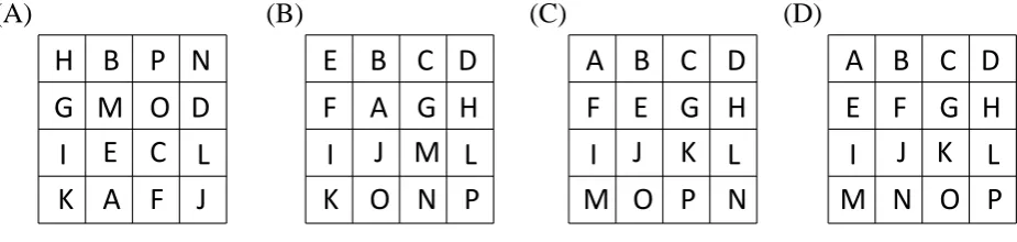
Discrete optimization problems are abundant in many fields of study, and have also started to begin to appear in the hy-drologic literature (Furman et al., 2004; Harmancioglu et al., 2004; Perrin et al., 2008; Kleidorfer et al., 2008; Neuman et al., 2011). Figure 1 illustrates a simple discrete parameter es-timation problem involving a tile puzzle. Each tile contains a different letter of the alphabet. The goal is to list the letters in the appropriate order. The solution to this problem is obvi-ous to a human, but not immediately clear to a computer. A search algorithm is therefore required to solve this problem.
If we assign numbers to each letter, A = 1, B = 2 and so forth, we could measure the distance from our initial guess to the actual solution, and iteratively refine this solution by sampling from a (discrete) proposal distribution. Many al-gorithms have been developed in the past decades to effi-ciently resolve problems of this kind. Yet, the main trust of these algorithms is on finding a single optimum solu-tion, without recourse to estimating the underlying posterior
uncertainty. For example, within the context of the travel-ing salesman problem many different routes will exist that only deviate marginally from the optimal solution. Brute force sampling of the search space can be used to assess all these plausible routes, but this seems rather inefficient. In-stead, a more intelligent search procedure is warranted that more efficiently samples the space of possible solutions. The goal of this paper therefore is to introduce theory and con-cepts of DREAM(D), a MCMC simulation algorithm that is especially designed to efficiently retrieve the posterior distribution of discrete and combinatorial search problems.
Figure 1a illustrates the application of DREAM(D) to the tile puzzle considered herein. The left panel depicts the ini-tial guess, whereas the remaining three panels (Fig. 1b–d) il-lustrate how DREAM(D)translates this random starting point into the final position of the letters. The next sections de-scribe the theory and concepts of DREAM(D) and present three different case studies.
3 DREAM(D)⇒DiffeRential Evolution Adaptive
Metropolis with Discrete Sampling
We now describe our new code, entitled DREAM(D), which uses DREAM as main building block. The algorithmic pa-rameters (with defaults in parentheses) areN(d) the number of chains,δ(1) the number of pairs used to generate the pro-posal, CRthe crossover probability (see later), K (10) the thinning rate in storing samples andTmax(106) the maximum
number of generations, typically so large that DREAM(D) automatically stops after convergence has been achieved.
Let X be aN×d-matrix with rows xi,i=1,...,N, that contain the current states of theN different Markov chains and that are iteratively updated in turn in the algorithm. The initial X= [Xt;t=0] is obtained by drawing N samples frompd(x), the prior distribution. Also, let S be an exter-nal archive that stores the elements of X at regular intervals. The initial population [Xt;t=0] is translated into a sam-ple from the posterior target distribution using the following pseudo code:
1. Sett←1
REPEATKtimes (POPULATION EVOLUTION) FORi←1,...,NDO (CHAIN EVOLUTION)
(a) Draw the number of dimensions to be updated,d0, from the binomial distribution with totaldand probabilityCR. Ifd0=0, setd0←1.
(b) Generate a new proposal, zi, for chaini,
zi=xi+
(1d+ed)γ (δ,d0)
δ X
j=1
Xr1(j )− δ X
n=1
Xr2(n)
+d d
(4)
where the functionk · kdrounds each elementj=1,...,d of the jump vector to the nearest integer. The various symbols have been defined after Eq. (3).
E
A
C
F
K
M
I
G
B
O
L
J
P
D
H
N
J
O
M
N
K
A
I
F
B
G
L
P
C
H
E
D
J
O
K
P
M
E
I
F
B
G
L
N
C
H
A
D
(A)
(B)
(C)
(D)
J
N
K
O
M
F
I
E
B
G
L
P
C
H
[image:4.595.67.530.64.174.2]A
D
Fig. 1. A 4×4 square tile puzzle with 16 different letters. The goal is to list the letters in order of the alphabet. Each letter is assigned a different integer value, and the resulting inverse problem is solved using DREAM(D). The left panel (a) presents the initial state, whereas the remaining three graphs (b–d) demonstrate how DREAM(D)iteratively solves this integer sampling problem.
and replace the corresponding proposal elementzji byxji.
The proposal zithus updatesd0elements of xionly.
(d) Compute p(zi) and accept the candidate points with Metropolis acceptance probability,α(xi,zi),
α(zi,xi)=1∧p(z i)
p(xi) (5)
(e) If accepted, move the chain to the candidate point, xi= zi, otherwise remain at the old location, xi.
END FOR (CHAIN EVOLUTION) END REPEAT (POPULATION EVOLUTION)
2. Append X to S.
3. Compute the Gelman-Rubin convergence diagnostic,Rˆj (Gel-man and Rubin, 1992) for each dimensionj=1,...,d using the last 50 % of the samples of S.
4. IfRˆj≤1.2 forj=1,...,d ort > Tmax, stop and go to step
5, otherwise sett←t+Kand go to POPULATION EVOLU-TION.
5. Summarize the posterior pdf using S after discarding the ini-tial and burn-in samples.
In words, DREAM(D) runs multiple different chains in parallel, and generates jumps in each individual chain using information from the location of the otherN−1 chains. The rounding operator, k · kd in Eq. (4) is used to enforce inte-ger values and accommodate discrete search problems. To speed up convergence to the target distribution, DREAM(D) estimates a distribution ofCRvalues during burn-in that fa-vors large jumps over smaller ones in each of theN chains. Details can be found in previous studies (Vrugt et al., 2008, 2009a,b, 2011b).
The transition kernel of DREAM(D)is especially designed for integer variables. This appears to be a major limita-tion as many discrete search problems involve non-integer variables. For instance, consider the discrete variablex1∈
[0,0.2,0.4,...,5]. We cannot sample this parameter with the proposal distribution presented in Eq. (4). A simple linear transformation of the search space,x1=0.2j;j∈ {0,...,25}
suffices to facilitate inference with DREAM(D). If appro-priate, a different transformation can be used for each in-dividual parameter. An extreme case would simultaneously involve discrete and continuous variables. This would con-stitute some combination of jumps generated with DREAM and DREAM(D).
3.1 DREAM(D)⇒detailed balance?
We are now left with a proof that DREAM(D)yields an in-variant distribution that is identical to the posterior target of interest. For this we need to demonstrate that the transi-tion kernel of DREAM maintains detailed balance, and thus results in a reversible Markov chain. In other words, the forwardp(xi→zi)and backwardp(zi→xi)jump should have equal probability at every single step in the chain. This is easy to proof for a standard RWM algorithm that uses a fixed proposal distribution. Hence, the forward and back-ward jump will exhibit equal probability. Yet, the jump dis-tribution used in DREAM(D)continuously changes scale and orientation en route to the posterior target distribution. This adaptation significantly enhances search efficiency, but does this also ensure reversibility of the sampled Markov chains?
Previous manuscripts have provided formal proofs of con-vergence of DREAM (Vrugt et al., 2008), DREAM(ZS) (Vrugt et al., 2011b), and MT-DREAM(ZS) (Laloy and Vrugt, 2011) to the appropriate limiting distribution. These proofs appear rather simple, but might not be easy to under-stand for those that are not directly familiar with the underly-ing statistics and mathematics. We therefore resort to a sim-ple hypothetical examsim-ple. Lets consider a two-dimensional discrete sampling problem withN=5 different chains, and thusγ=2.4/
√
0 1 2 3 4 5 0
1 2 3 4 5 6
6 7 7
r1
r2
x2
[image:5.595.47.289.66.303.2]x1 N = 5 different chains
Fig. 2. Illustration of detailed balance: two-dimensional parameter estimation problem withx1∈ [0,7]andx2∈ [0,7]. The color dots
denote the starting points of theN=5 different chains. The red square signifies the candidate point of the first chain and is created by selecting the blue chain asr1and green chain asr2. One step
later, after moving to the red square, the backward jump has equal probability, as there is an equal chance of drawingr1(green) andr2
(blue) in reversed order.
The candidate point of the first (purple) chain thus becomes:
zi= 2 2
+ 1.2
4 4
− 5 1
=
2 2 +
−1.2 3.6 =
1 6 (6) This proposal point is indicated in Fig. 2 with the red square. For the sake of this illustration, lets now assume that we ac-cept this candidate point, and transition the first chain to this new state.
We now need to demonstrate that the reverse jump has equal probability. This backward jump can be obtained by selecting the blue and green chain in the opposite order from the forward jump:
zi= 1 6
+ 1.2
5 1
− 4 4
=
1 6 +
1.2−3.6 =
2 2 (7) This point is exactly similar to the initial state of chain one prior to the forward jump. Apparently, the rounding operator used to sample integer values does not destroy detailed bal-ance. By samplingr1andr2from the remainingN−1 chains
with a uniform random number generator enforces symmetry of the proposal distribution. Indeed, the chance to selectr1
as chain two, andr2as chain four is equal to drawingr2=4,
andr2=2 in the reverse order. This also holds when ed, and dare drawn from their respective symmetric probability dis-tributions, and whenδ >1 andd >2. We leave this up to the reader. This concludes our proof of detailed balance.
A final remark is appropriate. Theoretically, it is possible that at least one of thed arguments of the rounding func-tion,k · kdhas a fractional part of.5. In this case, convention dictates to round down to the nearest integer. This directed rounding introduces a possible bias in jumping direction and thus strictly speaking violates detailed balance. The chance that this happens in practice is virtually zero. If nothing else, the stochastic nature of ed∼Ud(−b,b), andd∼Nd(0,b∗) will eliminate this possibility. But, in the rare event that any argument ofk · kd has a factional part of.5 we implement stochastic rounding to the nearest integer. This guarantees re-versibility of the Markov chains generated with DREAM(D).
3.2 Combinatorial search problems: proposal
distribution using position swapping
The parallel direction update of Eq. (4) works well for a range of discrete problems but is not necessary optimal for combinatorial problems in which the values of the final solution are known a-priori but not their order in the parameter vector. The topology of such search problems differs substantially from the Euclidean search problems considered hitherto. We therefore introduce an alternative jump distribution that creates candidate points by randomly swapping two coordinates in each individual chain.
PROPOSAL DISTRIBUTION: RANDOM SWAP FORi←1,...,NDO (CHAIN EVOLUTION)
1. Set zi=xi.
2. Randomly select two numbersj andk without replacement from{1,...,d}.
3. Swap thejthandkthcoordinates of zi;yji=xikandyki=xji. 4. Computeπ(zi)and accept the candidate points with
Metropo-lis acceptance probability,α(xi,zi).
5. If accepted, move the chain to the candidate point, xi=zi, otherwise remain at the old location, xi.
END FOR (CHAIN EVOLUTION) END RANDOM SWAP
In words, if the current state of the ith chain is given by xi =
x1i,...,xji,...,xki,...,xdi
then the candidate point becomes zi = x1i,...,xki,...,xji,...,xid where j,k are discrete uniformly sampled from {1,...,d} without re-placement. It is straightforward to see that this proposal distribution satisfies detailed balance as the forward and backward jump have equal probability.
the dissimilarities in coordinates of theN chains running in parallel. We implement this idea as follows:
PROPOSAL DISTRIBUTION: DIRECTED SWAP DO (CHAIN EVOLUTION)
1. Randomly select two chains, Xr1and Xr2without replacement
from the population X−r1,r2
t .
2. Find those coordinates of xr1 and xr2 that are dissimilar and
store these locations inζ.
3. Randomly permuteζ; setj=ζ1andk=ζ2.
4. Copy zr1 = xr1and zr2 = xr2.
5. Swap the elements of zr1;zr1
j =x r1
k andz r1
k =x r1
j .
6. Swap the elements of zr2;zr2
j =x r2
k andz r2
k =x r2
j . 7. Computeπ(zr1)andπ(zr2).
8. Accept both candidate points with probability, p(zr1,zr2)
equal to the product of their respective Metropolis ratios, p(zr1,zr2)=α(xr1,zr1)α(xr2,zr2).
9. If accepted, move both chains to their respective candidate points, xr1=zr1 and xr2=zr2; otherwise remain at their old
location, xr1and xr2.
END FOR (CHAIN EVOLUTION) END DIRECTED SWAP
This proposal distribution swaps location j and k within two different chains,r1,r2∈ {1,...,N}from the differences
in their coordinates. This update needs to be carefully implemented so that all different chains are updated only once. This requires that the number of chains, N >1 and hence is easiest to implement ifN is an even number. This approach considerably improves sampling efficiency, as will be illustrated later with a Sudoku puzzle.
The swap move is fully Markovian, that is, it uses only information from the current time for proposal generation, and retains detailed balanced with respect to π(·) because the reverse move is equally probable. If the swap is not fea-sible (less than two dissimilar coordinates), the current chain is simply sampled again. This is necessary to avoid com-plications with unequal probabilities of move types (Deni-son et al., 2002); the same trick is applied in reversible jump MCMC (Green, 1995). The restriction of the update to the dissimilar coordinates does not destroy detailed balance in any way; it just selects a subspace to sample on the basis of the current state. Coordinate swapping is especially power-ful for combinatorial problems. Based on some preliminary studies, we use a 90/10 % mix of directed and random swaps, respectively.
4 Case studies
We now present three different case studies with increasing complexity. The first study consists of a typical integer esti-mation problem, and involves a Sudoku puzzle. This puzzle
has become quite popular in the past 10 yr, and many news-papers, journals, and magazines around the world publish Sudokus for entertainment. This synthetic study illustrates the ability of DREAM(D) to help solve a relatively diffi-cult and high-dimensional combinatorial optimization prob-lem. The second study revisits a classical site characteriza-tion problem in vadose zone hydrology and involves infer-ence of the hydraulic properties of unsaturated soils from laboratory or in situ measured water retention data. This example demonstrates how DREAM(D) can be utilized to solve experimental design problems and guide measurement collection. The third and final study resolves discrete pa-rameters in a parsimonious lumped watershed model using observed daily discharge data from the Guadalupe River in Texas. The posterior distribution derived with DREAM(D)is compared against its counterpart derived with DREAM as-suming a continuous formulation of the model calibration problem.
4.1 The daily Sudoku
The first case study considers a Sudoku puzzle, a popular and widely practised integer estimation problem. We use this ex-ample to illustrate the ability of DREAM(D)to successfully find the optimum of a discrete search problem. The objective is to fill a 9×9 grid with numbers so that each column, each row, and each of the nine 3×3 sub-grids that make up the to-tal square contains the values of 1 to 9. The same integer may only appear once in each column and row of the 9×9 play-ing board includplay-ing in any of the nine 3×3 subregions. Each puzzle starts with a partially completed grid, and typically has a single (unique) solution. The puzzle was popularized in 1986 by the Japanese puzzle company Nikoli, under the name Sudoku, meaning single number (Hayes, 2006). Nowa-days, Sudoku puzzles are very popular, and widely practised by many millions of people throughout the world.
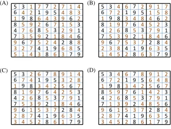
We consider the Sudoku puzzle in Fig. 3, taken from Wikipedia (http://en.wikipedia.org/wiki/Sudoku). The initial grid is depicted at the left-hand side, whereas the final solu-tion is presented at the right-hand side. In this particular puz-zle, the solution at 29 different cells is known, leaving us with
d=81−29=52 parameter values to be estimated. These parameters can take on values between 1 to 9. Figure 4 il-lustrates the sampled values of DREAM(D)at various stages during the search. A total ofN=20 different chains were used to search the parameter space, and the initial sample was created using random permutation of the available numbers. This ensures that each value of 1 to 9 appears only nine times in the grid. The log-likelihood function measures the sum of the horizontal, vertical and subgrid constraint violation.
(A) (B)
[image:7.595.159.436.64.204.2]From: Wikipedia
Fig. 3. The daily sudoku: (A) initial solution, and (B) final solution. The black numbers were given, whereas the solution numbers are marked in red.
(A)
(B)
(D)
(C)
5 3
6
9 8
7
1 9 5
6
3
1
6
3
6
2
8
8
4
7
6
4 1 9
8
7
9
5
2 8
1
2
4
1
9
5
6
7
5
3
7
6
2
4 3
2
9
5
7
1
7
4
7 5
7
4
2
1
9
3
5
3
2 4
6
9
1
8
1 4
3
2
2
5
9
4
8
8
8
6
3
5 3
6
9 8
7
1 9 5
6
3
1
6
3
6
2
8
8
4
7
6
4 1 9
8
7
9
5
2 8
4
2
7
1
9
1
6
2
3
5
6
3
2
4 8
7
9
5
4
1
9
1
7 5
8
5
3
4
9
2
1
2
3 7
6
4
5
5
1 7
8
7
2
2
9
4
8
4
3
6
3
5 3
6
9 8
7
1 9 5
6
3
1
6
3
6
2
8
8
4
7
6
4 1 9
8
7
9
5
2 8
2
4
7
1
9
1
6
2
3
5
6
3
8
4 2
7
9
5
4
1
9
3
1 5
7
5
8
4
9
2
3
2
3 7
6
5
2
2
1 4
8
7
7
5
9
4
8
4
3
6
1
5 3
6
9 8
7
1 9 5
6
3
1
6
3
6
2
8
8
4
7
6
4 1 9
8
7
9
5
2 8
4
2
7
1
9
5
6
2
3
1
6
3
8
4 2
7
9
5
1
4
9
6
1 5
7
5
8
4
9
2
3
2
3 7
6
5
4
4
1 2
8
7
7
2
9
5
8
4
3
6
1
Fig. 4. Sudoku puzzle: evolution of the DREAM(D)sampled parameter space to the posterior distribution: (A) typical starting solution, (B) intermediate solution, (C) nearly final solution, and (D) final solution.
violation of the constraints. Figure 4b displays the state of the same chain after about 25 000 function evaluations. The solution has improved considerably, but still contains sev-eral noticeable deviations from the actual solution. The third panel in Fig. 4c, derived after about 50 000 Sudoku evalu-ations is a further refinement of the solution presented in Fig. 4b. A few important swaps have been introduced that further reduce the constraint violation. Finally, after about 100 000 samples, Fig. 4d illustrates that the puzzle has been successfully solved.
[image:7.595.129.467.262.517.2]If our sole interest is in finding the optimum solution of a discrete search problem, then significant efficiency gains can be achieved with DREAM(D) by relaxing the assump-tion of detailed balance of the sampled Markov chains. For instance, if we modify the directed swap in DREAM(D) so that each candidate point is accepted/rejected based on its own Metropolis ratio independently of the associated move of the corresponding chain, then far fewer function evalua-tions would be needed to solve the Sudoku puzzle. The con-sequence of such non-Markovian adaptation, however is that the algorithm no longer adequately samples the underlying target distribution.
4.2 Optimal experimental design for soil hydraulic
characterization
The second case study considers a common problem in va-dose zone hydrology and involves characterization of the hy-draulic properties of variably saturated soils. This serves to demonstrate the ability of DREAM(D)to guide experimental data collection and help determine which soil water retention measurements to collect. We assume the capillary pressure-saturation relationship of (van Genuchten, 1980):
θ (h)=θr+(θs−θr)1+(αh)n −m
(8) whereθ(cm3cm−3) is the volumetric water content,h(cm) denotes the soil water pressure head,θs (θr) (cm3cm−3) sig-nifies the saturated (residual) water content,α(cm−1) andn
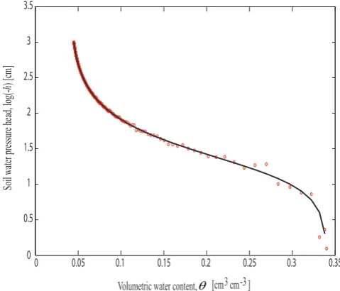
(-) are coefficients that determine the shape of the water re-tention function, andm=1−1/n. A synthetic data set of water retention observations was created for a sandy soil by evaluating Eq. (8) for a given set of pressure head values. The soil water pressure head was discretized intoM=501 equidistant points betweenh=0 (saturation) andh= −1000 (cm), and the correspondingθ (h)curve is plotted in Fig. 5 with a solid black line. Then, the soil water pressure head observations are corrupted with a normally distributed er-ror,h←N (h,2)to represent the combined effect of mea-surement error and soil inhomogeneity. The final data set is depicted with the circles in Fig. 5.
From this data set ofM=501 water retention measure-ments we now use DREAM(D) to find those four(h,θ (h)) observations that are most informative and best constrain the hydraulic properties, x= [θs,θr,α,n]of the sandy soil under consideration. For each selected combination of four differ-ent(h,θ (h))measurements in DREAM(D) we estimate the corresponding values of x by nonlinear minimization using the Nelder-Mead Simplex algorithm. The hydraulic param-eters obtained this way are then used to predict the water retention curve for the entire range of pressure head values considered in Fig. 5. A standard squared-deviation likelihood function is subsequently used to calculateπ(x)in step (d) of the pseudo code of DREAM(D)and summarize the informa-tion content for each selected set of four(h,θ (h)) observa-tions. We use the standard settings of DREAM(D) and run
0 0.05 0.1 0.15 0.2 0.25 0.3 0.35
0 0.5
1 1.5
2 2.5
3 3.5
Volumetric water content, [cm3 cm-3]
Soil water pressure head,
log(-h
) [cm]
[image:8.595.306.546.64.269.2]θ
Fig. 5. Synthetic soil water retention curve of the sandy soil, and the effect of data error.
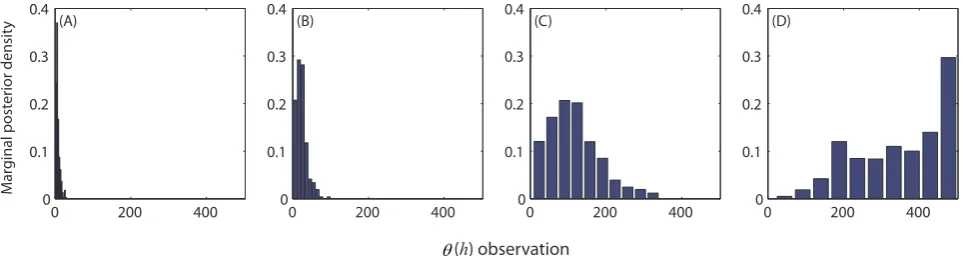
N=10 different Markov chains in parallel to search the dis-crete measurement space. About 10 000 function evaluations were required to reach convergence to a limiting distribution. Figure 6 presents the results of our analysis and plots histograms of the DREAM(D) derived posterior measure-ment samples after sorting each combination in increasing order. The marginal posterior distributions appear clustered around distinctly different soil water pressure head values. This includes soil water pressure head measurements around (Fig. 6a)h=0, (Fig. 6b)h= −40, (Fig. 6c)h= −220, and (Fig. 6d)h= −1000 cm respectively. Indeed, the most infor-mative(h,θ (h))observations are found close to saturation, around the air-entry value of the sandy soil, at the inflec-tion point of the water reteninflec-tion funcinflec-tion, and in the very dry moisture range. The location of these most informa-tiveθ (h)measurements matches very well with our previ-ous findings (Vrugt et al., 2002) and are in agreement with the dynamic behavior of the marginal sensitivity coefficients,
∂θ/∂θs, ∂θ/∂α, ∂θ/∂n, and ∂θ/∂θr derived from the par-tial derivatives of Eq. (8). A similar pattern is observed for loamy and clayey soils (not shown herein), but the second, third and last observation depicted in Fig. 4b–d move to-wards lower soil water pressure head values, consistent with the increased water holding capacity of these more fine tex-tured soils. An accurate soil hydraulic characterization thus requires water retention measurements that span the entire range of soil moisture values.
0 200 400 0
0.1 0.2 0.3 0.4
(A)
(h) observation
M
ar
ginal post
er
ior densit
y
0 200 400
0 0.1 0.2 0.3 0.4
(B)
0 200 400
0 0.1 0.2 0.3 0.4
(C)
0 200 400
0 0.1 0.2 0.3 0.4
(D)
[image:9.595.57.539.63.191.2]θ
Fig. 6. Histograms of the posterior samples generated with DREAM(D). The most informative soil water pressure head measurements are somewhat clustered at different moisture values that range from saturation (left plot) to the dry end (right plot). The x-axis indexes the observations[1,...,501].
for a redundancy in information content. This is an in-teresting finding, and explains why the parameters n and
θr are often found to be highly correlated in the fitting of water retention curves. The posterior spread derived with DREAM(D)is hence a useful byproduct to analyze measure-ment uniqueness, and determine the information content of experimental data.
4.3 Watershed model calibration using discrete
parameter estimation
The third and final case study involves flood forecasting, and consists of the calibration of a mildly complex lumped water-shed model using historical data from the Guadalupe River at Spring Branch, Texas. This is the driest of the 12 MOPEX basins described in the study of Duan et al. (2006). The model structure and hydrologic process representations are found in Schoups and Vrugt (2010). The model transforms rainfall into runoff at the watershed outlet using explicit pro-cess descriptions of interception, throughfall, evaporation, runoff generation, percolation, and surface and subsurface routing. Table 1 summarizes the seven different model pa-rameters, and their prior uncertainty ranges. Each parame-ter is discretized equidistantly in 250 inparame-tervals with respec-tive step size listed in the last column at the right hand side. This gridding is necessary to create a non-continuous, dis-crete, parameter estimation problem. Unlike the previous case study in which integer values are sampled only, this par-ticular study (mostly) involves non-integer values.
Daily discharge, mean areal precipitation, and mean areal potential evapotranspiration were derived from Duan et al. (2006) and used for model calibration. Details about the basin, experimental data, and likelihood function can be found there, and will not be discussed herein. The same model and data was used in a previous study (Schoups and Vrugt, 2010), and used to introduce a generalized likelihood function for heteroscedastic, non-Gaussian, and correlated (streamflow) prediction errors.
Figure 7 presents histograms of the marginal distribu-tion of a few selected hydrologic model parameters using five years of observed daily discharge data. The top panel presents the results of DREAM(D), whereas the bottom panel presents the results for a continuous parameter space. These histograms were derived by separately running DREAM for the same data set and model. Notice the close agreement between the histograms derived with both MCMC methods. This is a testament to the ability of DREAM(D) to success-fully solve discrete posterior parameter estimation problems. The influence of gridding is hardly noticeable, but becomes apparent if we use at least 25 bins to represent the marginal density (not shown herein).
To better illustrate the effect of discretization, please con-sider Fig. 8 that presents two-dimensional scatter plots of the DREAM(D)derived posterior samples for a few selected pa-rameter pairs. The bottom panel shows similar plots but then assuming continuity of the parameter space. The effect of gridding is immediately apparent. Whereas the original bi-variate scatter plots sample the parameter space in a (blood-stain) spatter pattern, two-dimensional plots of the posterior samples derived with DREAM(D) exhibit an obvious grid pattern with horizontally and vertically aligned points. The posterior samples take on discrete values with a distance be-tween subsequent points that is similar to the intervals listed in Table 1. Despite this difference in sampling pattern, the shape of the DREAM and DREAM(D)derived bivariate scat-ter plots are very similar, commensurate with the covariance structure of the posterior distribution. The results presented in Fig. 7 inspire confidence in the ability of DREAM(D) to solve noncontinuous posterior sampling problems.
Table 1. Prior Uncertainty Ranges of Hydrologic and Error Model Parameters.
Parameter Symbol Minimum Maximum Units Step size
Maximum interception Imax 0 10 mm 0.02
Soil water storage capacity Smax 10 1000 mm 1.98
Maximum percolation rate Qmax 0 100 mm d−1 0.20
Evaporation parameter αE 0 100 – 0.20
Runoff parameter αF −10 10 – 0.04
Time constant, fast reservoir KF 0 10 days 0.02
Time constant, slow reservoir KS 0 150 days 0.30
Heteroscedasticity intercept σ0 0 1 mm d−1 0.002
Heteroscedasticity slope σ1 0 1 – 0.002
Autocorrelation coefficient φ1 0 1 – 0.002
Kurtosis parameter β −1 1 – 0.004
0 2 4 6
0.1 0.2 0.3
Post
er
ior densit
y
(A)
40 60 80
0.1 0.2 0.3 (B)
0.84 0.86 0.88 0.1
0.2 0.3 (C)
DREA
M
(D)
0 2 4 6
0.1 0.2 0.3
Post
er
ior densit
y
Imax
(D)
40 60 80
0.1 0.2 0.3
KS (E)
0.84 0.86 0.88 0.1
0.2 0.3
1
(F)
DREA
M
φ
Fig. 7. Histogram of the DREAM(D)derived marginal posterior distributions of the (A)Imax, (B)KS, and (C)φ1rainfall – runoff and error
model parameters (in red). For convenience, only a few parameters are plotted. To benchmark the results of DREAM(D)the bottom panel illustrates the results for DREAM (in blue), with the common assumption of a continuous parameter space.
and details can be found in that publication. It is interest-ing to observe that the maximum log-likelihood value of 543 found with DREAM(D) is somewhat larger than its coun-terpart estimated with DREAM (540). This difference was consistently observed for multiple different trials with both MCMC algorithms.
[image:10.595.71.525.130.541.2]Fig. 8. Two-dimensional scatter plots of the DREAM(D)derived posterior samples (top panel: red), and corresponding bivariate samples estimated with DREAM (bottom panel: blue). Only a few parameter pairs are shown as this is sufficient to illustrate the similarity of the sampled distributions.
1 2 3 4 5
R-sta
tistic
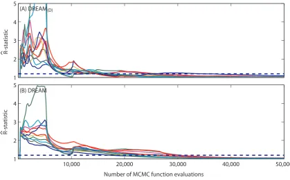
(A) DREAM (D)
10,000 20,000 30,000 40,000 50,000
1 2 3 4 5
R-sta
tistic
Number of MCMC function evaluations (B) DREAM
[image:11.595.85.505.389.649.2]convergence speed for both algorithms is strikingly similar. Both MCMC methods require about 30 000 model evalua-tions to converge to a limiting distribution. Although grid-ding significantly reduces the size of the feasible parameter space, an approximately similar number of function evalua-tions remains necessary to explore the posterior target dis-tribution. Our experience with models involving a much higher parameter dimensionality demonstrate considerable enhancements in efficiency (sometimes dramatically) when sampling in the discretized rather than continuous space. Discretization might therefore provide a practical solution to speed up search efficiency for insensitive parameters. Further research on this topic is warranted.
5 Conclusions
In the past decade much progress has been made in the devel-opment of sampling algorithms for statistical inference of the posterior parameter distribution. The typical assumption in this work is that the parameters are continuous and can take on any value within their upper and lower bounds. Unfor-tunately, such algorithms typically do not work for discrete parameter estimation problems. Such problems are abundant in many fields of study, and therefore of considerable the-oretical and practical interest. Examples include selecting among different measurement locations in the design of op-timal experimental strategies, finding the best members of an ensemble of predictors, and more generally discrete model calibration problems. Here, we have introduced a discrete MCMC simulation algorithm that is especially designed to solve non-continuous and combinatorial posterior sampling problems. This method, entitled DREAM(D) uses DREAM as its main building block, yet uses a modified proposal dis-tribution to facilitate solve discrete sampling problems. The DREAM(D)algorithm maintains detailed balance and ergod-icity, and receives good performance across a range of prob-lems involving a Sudoku puzzle, soil water retention function and discrete rainfall - runoff model calibration problem.
The theory developed herein is easily implementable in DREAM(ZS) (Vrugt et al., 2011b) and MT-DREAM(ZS) (Laloy and Vrugt, 2011), which provides a venue to fur-ther increase the efficiency of MCMC simulation. The DREAM(D) code is written in MATLAB and is available upon request ([email protected]).
Acknowledgements. We gratefully acknowledge the helpful com-ments of Christian Robert, Bettina Schaefli and one anonymous reviewer. Computer support, provided by the SARA center for par-allel computing at the University of Amsterdam, The Netherlands, is highly appreciated.
Edited by: E. Morin
References
Box, G. E. P. and Tiao, G. C.: Bayesian Inference in Statistical Analyses Addison-Wesley-Longman, Reading, Massachusetts, 1973.
Denison, D. G. T., Holmes, C. C., Mallick, B. K., and Smith, A. F. M.: Bayesian methods for nonlinear classification and regression, John Wiley & Sons, Chicester, 2002.
Duan, Q., Gupta, V. K., and Sorooshian, S.: Effective and efficient global optimization for conceptual rainfall-runoff models, Water Resour. Res., 28, 1015–1031, 1992.
Duan, Q., Schaake, J., Andr´eassian, V., Franks, S., Goteti, G., Gupta, H. V., Gusev, Y. M., Habets, F., Hall, A., Hay, L., Hogue, T., Huang, M., Leavesley, G., Liang, X., Nasonova, O. N., Noil-han, J., Oudin, L., Sorooshian, S., Wagener, T., and Wood, E. F.: Model Parameter Estimation Experiment (MOPEX): An overview of science strategy and major results from the second and third workshops, J. Hydrol., 320, 3–17, 2006.
Furman, A., Ferr´e, T. P. A., and Warrick, A. W.: Optimization of ERT surveys for monitoring transient hydrological events using perturbation sensitivity and genetic algorithms, Vadose Zone J., 3, 1230–1239, 2004.
Gelfand, A. E. and Smith, A. F.: Sampling based approaches to calculating marginal densities, J. Am. Stat. Assoc., 85, 398–409, 1990.
Gelman, A. G. and Rubin, D. B.: Inference from iterative simula-tion using multiple sequences, Stat. Sci., 7, 457–472, 1992. Gilks, W. R. and Roberts, G. O.: Strategies for improving MCMC,
in: Markov Chain Monte Carlo in Practice, edited by: Gilks, W. R., Richardson, S., and Spiegelhalter, D. J., Chapman & Hall, London, 89–114, 1996.
Gilks, W. R., Roberts, G. O., and George, E. I.: Adaptive direction sampling, Statistician, 43, 179–189, 1994.
Green, P. J.: Reversible Jump Markov Chain Monte Carlo Compu-tation and Bayesian Model Determination, Biometrika, 82, 711– 732, 1995.
Hastings, W. K.: Monte Carlo sampling methods using Markov chains and their applications, Biometrika, 57, 97–109, 1970. Haario, H., Saksman, E., and Tamminen, J.: Adaptive proposal
dis-tribution for random walk Metropolis algorithm, Computation. Stat., 14, 375–395, 1999.
Haario, H., Saksman, E., and Tamminen, J.: An adaptive Metropo-lis algorithm, Bernoulli, 7, 223–242, 2001.
Haario, H., Saksman, E., and Tamminen, J.: Componentwise adaptation for high dimensional MCMC, Computation. Stat., 20, 265–274, 2005.
Haario, H., Laine, M., Mira, A., and Saksman, E.: DRAM: Effi-cient adaptive MCMC, Stat. Comput., 16, 339–354, 2006. Harmancioglu, N. B., Icaga, Y., and Gul, A.: The use of an
opti-mization method in assessment of water quality sampling sites, European Water, 5/6, 25–35, 2004.
Hayes, B.: Unwed numbers, American Scientist, 94, 12–15, doi:10.1511/2006.1.12, 2006.
Kavetski, D., Kuczera, G., and Franks, S. W.: Bayesian analysis of input uncertainty in hydrologic modeling: 2. Application, Water Resour. Res., 42, W03408, doi:10.1029/2005WR004376, 2006. Kleidorfer, M., M¨oderl, M., Fach, S., and Rauch, W.:
Krink, T., Mittnik, S., and Paterlini, S.: Differential Evolution and Combinatorial Search for Constrained Index Tracking, Center for Studies in Banking and Finance, 09032, Universita di Modena e Reggio Emilia, Facolt`di Economia “Marco Biagi”, 2009. Kuczera, G., Kavetski, D., Franks, F. W., and Thyer, M. T.:
To-wards a Bayesian total error analysis of conceptual rainfall-runoff models: Characterising model error using storm-dependent parameters, J. Hydrol., 331, 161–177, 2006.
Laloy, E. and Vrugt, J. A.: High-dimensional posterior explo-ration of hydrologic models using multi-try DREAM(ZS) and high performance computing, Water Resour. Res., in review, doi:2011WR010608RR, 2011.
Metropolis, N., Rosenbluth, A. W., Rosenbluth, M. N., Teller, A. H., and Teller, E.: Equation of state calculations by fast computing machines, J. Chem. Phys., 21, 1087–1092, 1953.
Neuman, S. P., Xue, L., Ye, M., and Lu, D.: Bayesian analy-sis of data-worth considering model and parameter uncertain-ties, Adv. Water Resour., doi:10.1016/j.advwatres.2011.02.007, in press, 2011.
Perrin, C., Andr´eassian, V., Rojas Serna, C., Mathevet, T., and Le Moine, N.: Discrete parameterization of hydro-logical models: Evaluating the use of parameter sets li-braries over 900 catchments, Water Resour. Res., 44, W08447, doi:10.1029/2007WR006579, 2008.
Price, K. V., Storn, R. M., and Lampinen, J. A.: Differential Evo-lution, A Practical Approach to Global Optimization, Springer, Berlin, 2005.
Roberts, G. O. and Gilks, W. R.: Convergence of adaptive direction sampling, J. Multivariate Anal., 49, 287–298, 1994.
Roberts, G. O. and Rosenthal, J. S.: Coupling and ergodicity of adaptive Markov chain Monte Carlo algorithms, J. Appl. Probab., 44, 458–475, 2007.
Roberts, G. O. and Rosenthal, J. S.: Examples of adaptive MCMC, online manucript, available at: http://probability.ca/jeff/ftpdir/adaptex.pdf, 2008.
Roberts, G. O. and Rosenthal, J. S.: Optimal scaling for various Metropolis-Hastings algorithms, Statist. Sci., 16, 351–367, 2001. Schaefli, B., Talamba, D. B., and Musy, A.: Quantifying hydrolog-ical modeling errors through a mixture of normal distributions, J. Hydrol., 332, 303–315, 2007.
Schoups, G. and Vrugt, J. A.: A formal likelihood function for pa-rameter and predictive inference of hydrologic models with cor-related, heteroscedastic and non-gaussian errors, Water Resour. Res., 46, W10531, doi:10.1029/2009WR008933, 2010. Smith, T. J. and Marshall, L. A.: Bayesian methods in
hydro-logic modeling: A study of recent advancements in Markov chain Monte Carlo techniques, Water Resour. Res., 44, W00B05, doi:10.1029/2007WR006705, 2008.
Sorooshian, S. and Dracup, J. A.: Stochastic parameter estima-tion procedures for hydrologic rainfall-runoff models: correlated and heteroscedastic error cases, Water Resour. Res., 16, 430– 442, doi:10.1029/WR016i002p00430, 1980.
Storn, R. and Price, K.: Differential evolution a simple and efficient heuristic for global optimization over continuous spaces, Global Optimization, 11, pp. 341–359, 1997.
Ter Braak, C. J. F.: A Markov chain Monte Carlo version of the ge-netic algorithm differential evolution: easy Bayesian computing for real parameter spaces, Stat. Comput., 16, 239–249, 2006. Ter Braak, C. J. F. and Vrugt, J. A.: Differential evolution Markov
chain with snooker updater and fewer chains, Stat. Comput., 16, 239–249, doi:10.1007/s11222-008-9104-9, 2008.
van Genuchten, M. Th.: A closed-form equation for predicting the hydraulic conductivity of unsaturated soils, Soil Sci. Soc. Am. J., 44, 892–898, 1980.
Vrugt, J. A., Bouten, W., Gupta, H. V., and Sorooshian, S.: Toward improved identifiability of hydrologic model parameters: the in-formation content of experimental data, Water Resour. Res., 38, 1312, doi:10.1029/2001WR001118, 2002.
Vrugt, J. A., Gupta, H. V., Bouten, W., and Sorooshian, S.: A shuffled complex evolution metropolis algorithm for optimiza-tion and uncertainty assessment of hydrologic model parame-ters, Water Resour. Res., 39, 1–14, doi:10.1029/2002WR001642, 2003.
Vrugt, J. A., ter Braak, C. J. F., Clark, M. P., Hyman, J. M., and Robinson, B. A.: Treatment of input uncertainty in hy-drologic modeling: Doing hydrology backward with Markov chain Monte Carlo simulation, Water Resour. Res., 44, W00B09, doi:10.1029/2007WR006720, 2008.
Vrugt, J. A., ter Braak, C. J. F., Diks, C. G. H., Higdon, D., Robinson, B. A., and Hyman, J. M.: Accelerating Markov chain Monte Carlo simulation by differential evolution with self-adaptive randomized subspace sampling, I. J. Nonlin. Sci. Num., 10, 271–288, 2009a.
Vrugt, J. A., ter Braak, C. J. F., Gupta, H. V., and Robinson, B. A.: Equifinality of formal (DREAM) and informal (GLUE) Bayesian approaches in hydrologic modeling?, Stoch. Env. Res. Risk A., 23, 1011–1026, doi:10.1007/s00477-008-0274-y, 2009b. Vrugt, J. A., Laloy, E., and ter Braak, C. J. F.: Differential
![Fig. 2. Illustration of detailed balance: two-dimensional parameterestimation problem with x1 ∈ [0,7] and x2 ∈ [0,7]](https://thumb-us.123doks.com/thumbv2/123dok_us/9262810.995376/5.595.47.289.66.303/fig-illustration-detailed-balance-dimensional-parameterestimation-problem-x.webp)