www.hydrol-earth-syst-sci.net/20/2047/2016/ doi:10.5194/hess-20-2047-2016
© Author(s) 2016. CC Attribution 3.0 License.
HYPERstream: a multi-scale framework for streamflow routing in
large-scale hydrological model
Sebastiano Piccolroaz1, Michele Di Lazzaro2, Antonio Zarlenga2, Bruno Majone1, Alberto Bellin1, and Aldo Fiori2
1Department of Civil, Environmental, and Mechanical Engineering, University of Trento, via Mesiano 77,
38122 Trento, Italy
2Department of Engineering, Roma Tre University, Via Vito Volterra 62, 00146 Rome, Italy Correspondence to:Sebastiano Piccolroaz ([email protected])
Received: 24 August 2015 – Published in Hydrol. Earth Syst. Sci. Discuss.: 4 September 2015 Revised: 8 January 2016 – Accepted: 4 May 2016 – Published: 24 May 2016
Abstract.We present HYPERstream, an innovative stream-flow routing scheme based on the width function instanta-neous unit hydrograph (WFIUH) theory, which is specifically designed to facilitate coupling with weather forecasting and climate models. The proposed routing scheme preserves ge-omorphological dispersion of the river network when deal-ing with horizontal hydrological fluxes, irrespective of the computational grid size inherited from the overlaying climate model providing the meteorological forcing. This is achieved by simulating routing within the river network through suit-able transfer functions obtained by applying the WFIUH the-ory to the desired level of detail. The underlying principle is similar to the block-effective dispersion employed in ground-water hydrology, with the transfer functions used to repre-sent the effect on streamflow of morphological heterogene-ity at scales smaller than the computational grid. Transfer functions are constructed for each grid cell with respect to the nodes of the network where streamflow is simulated, by taking advantage of the detailed morphological information contained in the digital elevation model (DEM) of the zone of interest. These characteristics make HYPERstream well suited for multi-scale applications, ranging from catchment up to continental scale, and to investigate extreme events (e.g., floods) that require an accurate description of routing through the river network. The routing scheme enjoys parsi-mony in the adopted parametrization and computational effi-ciency, leading to a dramatic reduction of the computational effort with respect to full-gridded models at comparable level of accuracy. HYPERstream is designed with a simple and flexible modular structure that allows for the selection of any rainfall-runoff model to be coupled with the routing scheme
and the choice of different hillslope processes to be repre-sented, and it makes the framework particularly suitable to massive parallelization, customization according to the spe-cific user needs and preferences, and continuous develop-ment and improvedevelop-ments.
1 Introduction
The increasing pressures on freshwater resources originating from a multitude of complex and interacting factors led in recent years to a growing need of tools able to provide water resources information at regional to global scales (see, e.g., Archfield et al. (2015) for a commentary). Overall, this fos-tered new developments in large-scale hydrological models as a component of more comprehensive, and complex, Earth system models (ESMs). Manabe (1969) was the first to add a land component in a climate model. His work prompted the development of a first generation of global circulation models and a parallel development of land surface models (LSMs) for hydrological applications (see Haddeland et al. (2011) and Prentice et al. (2015) for a comprehensive re-view). Land surface models are developed with the intent of providing a realistic and detailed representation of ver-tical water, energy and CO2 fluxes, with the perspective to
(Niu et al., 2011), WEHY-HCM (Kavvas et al., 2013), and CLM (Oleson et al., 2013) are examples of LSMs, while MacPDM (Arnell, 1999), WBM (Vörösmarty et al., 1998), WGHM (Döll et al., 2003), WASMOD-M (Widén-Nilsson et al., 2007), PCR-GLOBWB (Van Beek et al., 2011), LIS-FLOOD (van der Knijff et al., 2010), and mHM (Samaniego et al., 2010) can be classified as belonging to the category of LHMs. This classification notwithstanding, the boundary between these two categories is blurred since in their recent developments most of these models are converging to a com-prehensive representation of the terrestrial processes, in an attempt to increase realism, though this is often achieved at the expense of reliability and robustness (Prentice et al., 2015). However, at the current stage of development, both categories of models suffer from a discretization which is of-ten too coarse to represent routing in the river network with enough detail to capture geomorphological dispersion (Ri-naldo et al., 1991).
The hydrological component of both categories of mod-els, which for simplicity we indicate here as LHMs, relies on simplified conceptualizations and empirical upscaling proce-dures (Nazemi and Wheater, 2015), when dealing with het-erogeneities that characterize hydrological fluxes across a hi-erarchy of scales, ranging from the hillslope to the catchment and the continent. In addition, most of the available hydro-logical models inherit the grid approach from LSMs, which works fine for the vertical fluxes, but makes streamflow rout-ing grid dependent. The obvious consequence is the presence of inaccuracies in the representation of horizontal fluxes, less a very fine discretization is used, which however is un-tenable at large scales also for the currently available high-performance computational resources. Indeed, grid-based LHMs are typically applied with a spatial resolution ranging from 0.1◦ (ca. 11 km) to 0.5◦ (ca. 55 km), which has been proven to be insufficient to capture geomorphological dis-persion and travel time distribution at the level of accuracy needed to model horizontal fluxes. This is particularly signif-icant at intermediate scales, i.e., scales of the order of thou-sand or tens of thouthou-sand km2 (Gong et al., 2009; Verzano et al., 2012), which are relevant in modeling flood events. The introduction of improved routing schemes to adequately resolve horizontal fluxes with an acceptable computational effort is therefore indicated as one of the priorities in ESMs, and in LHMs as well (Clark et al., 2015).
Hyper-resolution LHMs relying on global digital drainage networks at fine scales, such as HydroSHEDS at 90 m reso-lution (Lehner et al., 2008), represent a possible strategy to overcome the above limitations and obtain reliable estimates of horizontal fluxes (Wood et al., 2011). However, applying a LHM at a such fine discretization is difficult for the large computational cost associated with it, which becomes un-bearable when inversion is applied to infer model parameters from observational data. This burden is currently too high for LHMs adopting explicit hydrodynamic routing through the numerical solution of the mass and momentum
conserva-tion equaconserva-tions (i.e., the de Saint-Venant equaconserva-tions), but also for models adopting cell-by-cell routing algorithms based on mass conservation and relationships between river-channel storage and streamflows (Yamazaki et al., 2011; De Paiva et al., 2013). If modeling high flow events is the objective of the analysis an hourly, or smaller, timescale should be adopted, thereby further increasing the computational bur-den, with respect to the daily or monthly timescale typically adopted in large-scale simulations of water resources.
Mixed schemes in which routing is separated from runoff have also been employed (see, e.g., Gong et al., 2009, 2011; Wen et al., 2012; Lehner and Grill, 2013). HydroROUT is a vector-based routing scheme fully integrated with ArcGIS (ESRI, 2011) developed by Lehner and Grill (2013), in which streamflow is obtained by routing to the catchment outlet the surface runoff (as provided by an external runoff simu-lator to be coupled with the routing scheme) accumulated at the nodes of the network. Routing is performed by using a “plug-flow” routing scheme similar to that implemented by Whiteaker et al. (2006) and applied to the HydroSHEDS river network (Lehner et al., 2006).
Wen et al. (2012) proposed a multi-scale routing frame-work employing a probability density function (pdf) distri-bution for the overland flow path lengths lumping the ef-fect of unmodeled sub-grid variability in the parameters de-scribing the pdf. The kinematic wave routing method is then employed for both overland and channel flow simulations, thereby resulting in a highly computational demand, as al-ready discussed above. In addition, the routing scheme gen-erates streamflow only at the outlet of the catchment with-out the possibility to simulate streamflows at internal nodes, such as lakes, reservoirs or other infrastructures, while the use of response functions aggregated at the daily timescale limits the applicability to flood events occurring in large river basins, with the approach proposed by Gong et al. (2009, 2011).
repro-duction of horizontal water transfers. Here we refer to this as “perfect upscaling” to indicate that the proposed routing scheme keeps the network contribution inherently invariant with respect to the grid size of meteorological forcing: geo-morphological dispersion (Rinaldo et al., 1991) is preserved as it is derived from the morphological information embed-ded in the available digital elevation model (DEM). Scale in-variance is an important feature characterizing our modeling approach not enjoyed by grid-based LHMs, which rely on empirical upscaling procedures in order to represent unmod-eled geomorphological dispersion. Here perfect upscaling is presented for the case study of Upper Tiber (central Italy), where we show that our routing scheme does not entail any deterioration in the watershed width functions when consid-ering progressively coarser spatial resolutions.
An additional crucial aspect is the computational time ef-ficiency, which stems from the fact that the most demand-ing step of the procedure is the computation of the geomor-phological width functions, which is performed only once as an offline pre-processing procedure. This characteristic, cou-pled with easiness of parallelization and parsimony in pa-rameterization, inspired us to coin the name HYPERstream, where “HYPER” recalls that the proposed model is based on a “HighlY Parallelizable and scalablE Routing” scheme. Finally, HYPERstream is designed with a flexible and mod-ular structure which allows the coupling with any lumped or process-based formulation for infiltration and subsurface flow processes, while the simplicity and computational effi-ciency makes it an appealing tool for uncertainty assessment of the predictions, and in general for simulations conducted in a Monte Carlo framework.
This paper is organized as follows: Sect. 2 describes the multi-scale hydrological conceptual model; details of the pre-processing module and derivations of node specific width functions are provided in Sect. 3, with reference to the Upper Tiber case study. An example of application for two flood events is discussed in Sect. 3.3, and finally concluding re-marks are drawn in Sect. 4.
2 Model development
As stated in the Introduction, our aim is to develop a sim-ple, parsimonious and computationally efficient method for streamflow routing (with particular attention to floods) in large river basins. To this aim, we adopt different model-ing strategies for the river network and the associated hill-slopes (the land component introduced in Sect. 1): a lin-ear, geomorphologically based approach for the former, and a lumped formulation for the latter. We note that the land component can be decided without particular restrictions, de-pending only on the user’s needs and preferences. The pro-posed modeling framework reflects the current understand-ing of hydrological processes at the hillslope and watershed scales (see, e.g., Sivapalan, 2003).
ith macrocell
DEM cell
River network Node
k=1 aℓ 1
i=1 i=2 i=3
i
k=2 k=3
k=4
k=5 (1)
aℓ 1 (2)
= Lℓ 1 (2)
= τ
ℓ 1 (2) Lℓ 1
(1)
τ
ℓ 1 (1)
τ 1 3
A2 (3) A1
(3)
Catchment area (A)
D13
[image:3.612.319.535.65.328.2]Hillslope–channel transition site
Figure 1. Sketch of basin conceptualization: subdivision of the study area into macrocells and nodes (red dots). River network is subdivided into hillslope–channel transition sites (colored squared symbols) each associated with a pertaining hillslope areaa`k(i) (col-ored areas). For this simple case we considerN=9 macrocells and Nk=5 nodes. An example of two pathways characterized by the same lengthL(i)`k and travel timeτ`k(i)is also sketched.
The sketch of Fig. 1 displays the conceptual model adopted here. The modeled domainA, which can be of any size and may include any number of disconnected river net-works (for example, the sketch of Fig. 1 contains two river networks), is subdivided intoNmacrocells, each one charac-terized by a contributing areaA(i), such thatPNi=1A(i)=A. We emphasize that the genericA(i) does not need to coin-cide with the macrocell area; for instance this happens when the macrocell contains parts of neighbor watersheds (see the macrocells at the boundary of Fig. 1). There are no con-straints onA, except that it must cover all the watersheds of interest. For easiness of representation, in Fig. 1 macrocells are represented as squares, but this is not by any means a lim-itation of the model and irregular macrocells can be used if convenient in the application of the model. Indeed, size and geometry of the macrocells can be set to coincide with the gridding of the weather or climate model used to provide the input meteorological forcing.
identifi-cation of drainage direction and hillslope–channel separation (Tarboton et al., 1991; Montgomery and Foufoula-Georgiou, 1992) (see Sect. 3.2), the river networks are extracted and the hillslopes identified.
The area of the hillslopes changes through the domain, un-less identification of the river networks is performed by using a constant threshold area. The link between the hillslope and the channel is denoted as hillslope–channel transition site. As an example, a synthetic DEM grid is shown in Fig. 1 (25 DEM cells per macrocell) together with the identified river network. The figure shows also a few hillslopes (col-ored areas), each of them associated with the corresponding hillslope–channel transition site (colored squared symbols). Notice that in the example the brown hillslope is divided be-tween two macrocells (i=1,2), a common situation in our approach since the discretization of the domain into macro-cells may be arbitrary (i.e., it does not necessarily use to-pographic information, as is generally the case in weather forecasting or climate models).
The next step in the construction of the model is the iden-tification of theNk nodes where streamflow is simulated. In
the example of Fig. 1,Nk=5 nodes, identified by red bullets,
[image:4.612.307.504.182.237.2]are distributed within two networks. No limitations are im-posed to the number and position of these nodes, which rep-resent locations where streamflow is computed either to com-pare it with observational data, as part of the inversion proce-dure, or for other purposes, such as to verify flood protection structures (or the need to build them). Each macrocellimay feed one or more nodes; for instance, the macrocelli=3 in Fig. 1 includes contributing areas to nodesk=1 andk=2, with different routes. It may also occur that a macrocell con-tributes to the same nodekwith different routes, as for the case of macrocell i=2 which contributes to node k=1, through both hillslopes highlighted in green and brown.
We denote withA(i)k the area of macrocellicontributing to nodek, such thatPNk
k=1A (i) k =A
(i). Notice thatA(i) k =0 if
the macrocellidoes not contribute to nodek. The runoff gen-eration processes occurring at the hillslope scale can be mod-eled by using schemes of different level of complexity, from the simple SCS-CN method (U.S. Soil Conservation Service, 1964) to methods based on the solution of the Richards equa-tion, or one of its simplification (Clark et al., 2015), depend-ing on the objectives of the analysis.
Whatever the hillslope model, for the sake of generality hereafter we indicate withη(i)`k[L/T]the water discharge per unit area produced by the hillslope`of areaa(i)`k [L2], which belongs to the macrocelliand contributes to the streamflow at the closest downstream node k along the river network (for instance, the hillslope highlighted in green in Fig. 1 con-tributes to node k=1, which is the first node encountered moving downstream). The resulting water flow is triggered by rainfall or snowmelt and depends on the partitioning of hydrological fluxes at the hillslope scale, according to the
se-lected hillslope model and the hydrological processes that are simulated.
According to the above conceptual scheme, water flow produced by the hillslope enters the network system through the hillslope–channel transition site and is subsequently routed through it.
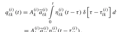
From this kinematic scheme, it follows that the streamflow contribution of the hillslope`, belonging to the macrocelli, to nodekcan be written as follows
q`k(i)(t )=A(i)k ea`k(i)
t Z
0
η(i)`k(t−τ ) δhτ−τlk(i)idτ
=A(i)k ea`k(i)η(i)`k(t−τ`k(i)) , (1) whereea`k(i)=a`k(i)/A(i)k [−] is the relative hillslope area, δ [1/T]is the Dirac delta function,τ`k(i)[T]is the travel time from the hillslope–channel transition site of the hillslope`to nodek, andt[T]is the current time.
Under the hypothesis that the stream velocityVc [L/T]
is constant through the network, the travel time assumes the following expression:τ`k(i)=L(i)`k/Vc, where L(i)`k is the
distance, measured along the network, from the hillslope– channel transition site of the hillslope` to the first down-stream nodek. The assumption of constantVcis crucial for
the linearity of the processes at the watershed scale, as stated at the beginning of this section. Equation (1) is consistent with the general conceptual framework used to derive the WFIUH by rescaling the geomorphological width function through a suitable constant velocity (Gupta et al., 1986; Mesa and Mifflin, 1986; Gupta and Mesa, 1988; Rodríguez-Iturbe and Rinaldo, 1997). We note that the assumption of con-stant channel velocity is supported by experimental measure-ments, especially for high flow conditions (see, e.g., Pilgrim, 1976, 1977). Additionally, stream hydrodynamic dispersion is neglected, owing to its small to negligible effect on the hydrological response, which has been demonstrated to be dominated by geomorphological dispersion already embed-ded into the rescaled width function (Rinaldo et al., 1991, 1995; Rodríguez-Iturbe and Rinaldo, 1997).
The streamflowqk(i)[L3/T]generated by macrocelliand contributing to the nodekis then obtained by summing up all the contributions stemming from the hillslopes of the macro-cell draining to the nodek:
qk(i)(t )=A(i)k X
` ea
(i) `k
t Z
0
η(i)`k(t−τ ) δhτ−τlk(i)id τ . (2)
qk(i)(t )=A(i)k
t Z
0
η(i)(t−τ ) fk(i)(τ ) dτ
=A(i)k η(i)∗fk(i)(t ) , (3) where fk(i)(τ )=P
`ea (i) `kδ
h
τ−L(i)`k/Vc i
is the probability density function (pdf) of the travel timeτ`k(i)weighted by the relative hillslope areaea`k(i). In Eq. (3) the asterisk denotes con-volution.
Finally, water discharge Qk(t )[L3/T] at the node k is
given by the sum of the direct contribution of each macrocell ito the node plus the contribution of the nodes upstream of k:
Qk(t )= N X
i=1
qk(i)(t )+
N X
i=1 Nkup X
j=1
qj(i) t−τj k, (4)
whereτj k=Dj k/Vcis the travel time from the node j,
lo-cated upstream ofk, to the nodek,Dj k is the distance
be-tween the two nodes, and Nkup is the number of nodes up-stream ofk.
In the first right-hand term of Eq. (4) summations are extended over all the macrocells, with the convention that qk(i)=0, becauseA(i)k =0, for all macrocells not contribut-ing, i.e., not connected through the network, to the nodek (the same applies for index j). Notice that, in the second right-hand term of Eq. (4) the streamflow computed at the nodej is rigidly translated to the nodekwith the delayτj k
depending on the distance between the two nodes, thereby neglecting again the effect of stream hydrodynamic disper-sion, as typically done in the WFIUH approach (see, e.g., Gupta et al., 1986; Van Der Tak and Bras, 1990; Botter and Rinaldo, 2003; Giannoni et al., 2005).
The above method is simple and computationally effec-tive. The underlying principle is similar to the block-effective dispersion employed in groundwater hydrology (see, e.g., Rubin et al., 1999; De Barros and Rubin, 2011), with the travel time pdf used to represent the effect on streamflow of morphological heterogeneity at scales smaller than the macrocell, with a lower cutoff given by the DEM scale. The linearity of the transfer processes at the scale of the network makes the algorithm easy to parallelize, making it promis-ing for large-scale applications at small timescales (i.e., with hourly or sub-hourly time steps). In principle, streamflow generated by a macrocell can be elaborated by a single pro-cessor (with the convolution of Eq. (3) being the most de-manding step), for the whole duration of the simulations, independently of the other processors. Then, the stream-flowQk(t )at the nodes of interest is further processed with
Eq. (4) when all processors terminated the elaboration of their macrocell. For the same reasons, this model is partic-ularly suited to multiple Monte Carlo runs (e.g., for param-eter estimation, uncertainty analysis, model or multi-scenario analysis). The main advantage of the method is that,
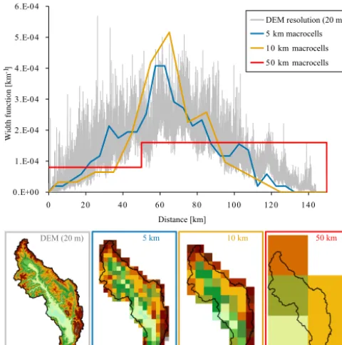
by design, it preserves the global geomorphological disper-sion of the basin, as calculated by the fine-grid DEM, no matter the size of the macrocells. Consequently, the upscal-ing of river network dispersion is perfectly resolved, with-out resorting to hyper-resolution numerical grids. This point shall be illustrated in the ensuing section. Spatial variabil-ity of precipitation, which indeed plays a fundamental role in shaping the hydrological response of river basins at inter-mediate spatial scale (i.e., beyond a few thousands of km2, see Nicótina et al., 2008; Volpi et al., 2012; Sapriza-Azuri et al., 2015), is in our scheme inherited from the companion climatic model and it is embedded in the hillslope produc-tion funcproduc-tionηaccording to the macrocell resolution. Sim-ilar approaches relying on distributed versions of geomor-phological response, but generally based on a partition of the watershed into natural or anthropogenic sub-basins and not focused on large-scale applications, can be found in Naden (1992), Moussa (1997), Rinaldo et al. (2006), Hallema et al. (2013), Hallema and Moussa (2014), Rigon et al. (2015), and Bellin et al. (2016).
Routing requires the definition of only a parameter, the channel velocityVc, which is a very parsimonious, yet
ef-fective, parametrization with respect to grid-based routing schemes. If the DEM resolution is high and the total domain Awhere the model is applied is large, the preprocessing step can be time-consuming; the effort is however compensated in the application of the model, particularly if the modeling activity is performed in a multiple run framework. We note that the only pre-processing operation required is the analy-sis of the DEM aimed at identifying the river network and the drainage characteristics of the river basin, and at computing the geomorphological width functions.
3 Description of the model features, with application to the Upper Tiber basin
3.1 Study area
(a)
(b)
(c)
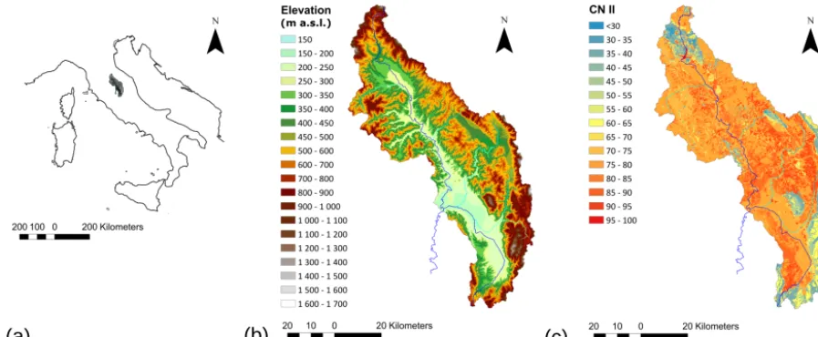
Figure 2.Maps showing(a)the location of the Upper Tiber river basin within the Italian Peninsula,(b)DEM of the watershed and(c) fine-scale land classification according to the CN II parameter.
However, high-permeability formations (calcareous lithol-ogy) are found in the upper part of the basin and on the east-ern divide.
Intense precipitation events are typically associated with humid frontal advection from the Mediterranean Sea and condensation due to the orographic uplift. Because of strong topographic gradients, headwaters experience intense rain-fall events, mostly occurring from autumn to spring, asso-ciated with frequent flood events. Substantial flood events have been also observed in the floodplain of the river (south-ern part) where most of population and economical activ-ities are clustered (Manfreda et al., 2014). Topography is represented through a 20 m resolution DEM provided by the Istituto Geografico Militare (IGM, available online at http://www.igmi.org/). Digital maps of land use and litho-logical characterization were supplied by the European Envi-ronmental Agency (Corine Land Cover project) and by Ital-ian Agency for Environmental Protection and Research (IS-PRA), respectively (maps not shown). Furthermore, land use classes from Corine classification and infiltration capacity es-timates were used to associate at each DEM cell a value of the curve number parameter (CNII, see Fig. 2c), which shall be used in the SCS-CN runoff model as described in Sect. 3.3.
3.2 Macrocell discretization, width functions derivation and perfect upscaling
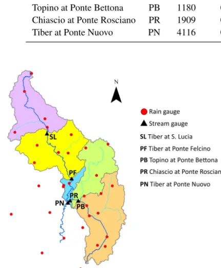
The control sections adopted for multi-site model validation (see Sect. 3.3) are located at five stream-gauge stations: Santa Lucia (SL), Ponte Felcino (PF), Ponte Bettona (PB), Ponte Rosciano (PR) and Ponte Nuovo (PN), with the latter be-ing the outlet of the river basin (see Fig. 3). Drainage area (ranging between 1000 and 4000 km2), longest flow path,
and other geomorphic characteristics of the sub-catchments identified by the five control nodes are reported in Table 1. The control nodes are located along the main course of the Tiber river and its two major tributaries (Chiascio and Topino rivers), and they are equipped with gauges registering water levels at 30 min time steps. Stage measurements in the pe-riod 1990–2000 together with validated stage–discharge re-lationships have been provided by the Hydrographic Service of Umbria Region (http://www.idrografico.regione.umbria. it). The meteorological forcing is described with half-hourly precipitation at 32 meteorological stations managed by the same institution. Figure 3 shows a map with the locations of the meteorological and stream gauging stations together with the subdivision of the watershed into the five inter-basin ar-eas.
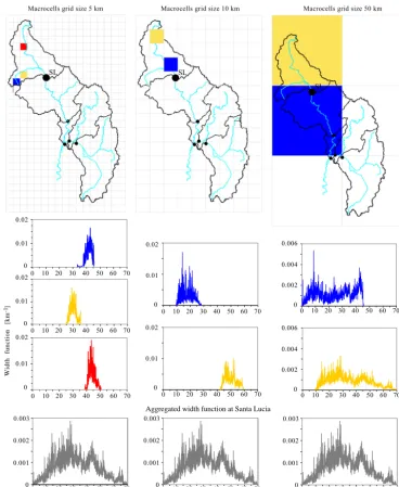
In the following the effect of spatial discretization on the hydrologic response is analyzed with reference to macro-cells of different dimensions. In particular, the study area was overlaid with macrocells of increasing size, from 1 to 150 km (the latter including the whole Upper Tiber river basin within a single macrocell), and corresponding to about 0.009 and 1.25◦, respectively. Domain discretization with macrocells of 5, 10 and 50 km is shown as an example in Fig. 4.
combi-Table 1.Main geomorphic characteristics of the inter-basin drainage areas within the Upper Tiber river basin (CV: coefficient of variation).
Basin ID Area Slope Channel length Statistics
(km2) (m m−1) Max (km) Mean (m) Variance (m2) CV (m m−1)
Tiber at Santa Lucia SL 932 0.009 66.1 32 482 2.03×10⁸ 0.44
Tiber at Ponte Felcino PF 2032 0.005 112.6 60 201 6.97×10⁸ 0.44
Topino at Ponte Bettona PB 1180 0.009 65.1 37 495 2.41×10⁸ 0.41
Chiascio at Ponte Rosciano PR 1909 0.007 92.9 48 477 4.74×10⁸ 0.45
[image:7.612.81.512.86.180.2]Tiber at Ponte Nuovo PN 4116 0.005 139.6 67 410 8.84×10⁸ 0.44
Figure 3.Map showing the subdivision of the watershed into five inter-basins, each one identified by a node where water discharge is computed (black triangles). The locations of the meteorological stations are also shown as colored dots.
nation of the threshold-slope area and the threshold-support area criteria (Di Lazzaro, 2009).
For a given resolution of the macrocell grid, it is thus pos-sible to derive the frequency distribution fk(i) of the flow path lengthsL(i)`kpertaining to macrocelliand connecting the hillslope–channel transition site of the hillslope`to the con-trol nodek(i.e., the macrocell-node specific width functions introduced in Sect. 2), which is the best possible approxima-tion of the width funcapproxima-tion, given the scale of the DEM.
Figure 4 shows as an example width functions constructed at the Santa Lucia node (upstream node on the main river course, see Fig. 3), for a few macrocells of size 5, 10, and 50 km, respectively. When the macrocell is small with re-spect to the sub-catchment, its width function is narrow, since it includes a reduced number of hillslopes. Conversely, when the macrocell is large enough to cover the entire catchment, its width function tends towards that of the sub-catchment. The first case is approached by the discretization with macrocells of 5 km (left panels in Fig. 4). The width
[image:7.612.61.277.143.404.2]0 10 20 30 40 50 60 70
0 10 20 30 40 50 60 70
0 10 20 30 40 50 60 70
Macrocells]grid]size]5]km Macrocells]grid]size]10]km Macrocells]grid]size]50]km
Distance][km]
0 0.002 0.003
0.001
0 10 20 30 40 50 60 70
Distance][km]
0 0.002 0.003
0.001
0 10 20 30 40 50 60 70
0 0.01 0.02
0 0.01 0.02
0 0.01 0.02
0 10 20 30 40 50 60 70
0 10 20 30 40 50 60 70
0 0.01 0.02
0 0.01 0.02
0 10 20 30 40 50 60 70
0 10 20 30 40 50 60 70
0 0.002 0.004 0.006 0 0.002 0.004 0.006
SL SL
SL
Distance][km]
0 0.002 0.003
0.001
0 10 20 30 40 50 60 70
Aggregated width function at Santa Lucia
W
id
th
fu
n
c
ti
o
n
[km ]
[image:8.612.114.482.63.511.2]-1
Figure 4.Width functions computed at the Santa Lucia (SL) control section for selected macrocells (colored lines) and for the whole sub-catchment (grey lines, panels at the bottom), considering grid sizes of 5, 10 and 50 km. The width function of the whole sub-sub-catchment is by design the same for the three spatial resolutions.
3.3 Application example
In this section we present an example of application of HY-PERstream for flood prediction in the Upper Tiber basin, with the purpose to illustrate its major computational and functional features. To focus on the routing scheme, the ex-ercise has been intentionally kept as simple as possible. In particular, the hillslope production function has been de-fined by combining the widely used SCS-CN method (U.S. Soil Conservation Service, 1964) for runoff simulation with a linear reservoir model describing the travel time distri-bution within the hillslope (Rodríguez-Iturbe and Rinaldo,
0.E+00 1.E-04 2.E-04 3.E-04 4.E-04 5.E-04 6.E-04
0 20 40 60 80 100 120 140
Distancee[km]
DEMeresolutione(20em) 5ekmemacrocells 10ekm emacrocells 50ekm emacrocells
50ekm
10ekm
5ekm DEMe(20em)
Width function [km ]
[image:9.612.46.286.66.307.2]-1
Figure 5.Width functions of the Upper Tiber river basin at Ponte Nuovo (PN) outlet (4116 km2) obtained aggregating the original 20 m DEM to 5 (blue), 10 (orange), and 50 (red) km. The width function derived from the original 20 m DEM is also shown (grey). Aggregated DEMs with grid size of 5, 10, and 50 km are shown in the lower part of the figure.
scale. In this case, rescaling may be obtained by using a hill-slope specific velocityV`Vc.
At the hillslope scale runoff is computed by using the clas-sic SCS-CN scheme:
Ri(t )=
Pi(t )−Ia,i 2
Pi(t )+cSSi−Ia,i
, (5)
wherePi(t )[L]andRi(t )[L]are the cumulative rainfall and
the cumulative runoff, respectively, at timet, both assumed uniform within the macrocelli. In addition,Si[L]is the soil
potential maximum infiltration (defined constant within each macrocell and estimated on the basis of the map of CNII shown in Fig. 2c), Ia=αcSS[L] is the initial abstraction,
withα <1 [–] introduced to represent the initial abstraction as a fraction of the maximum infiltration, andcS[–] is a
mul-tiplicative factor accounting for uncertainty in the identifica-tion ofS.
Therefore, the effective rainfall intensitypi[L/T]at time
t can be computed as follows: pi(t )=
Ri(t )−Ri(t−1t )
1 t , (6)
and Eq. (5) is applied at discrete times, according to the time step1t.
The specific water flux produced by the hillslopes of the macrocellican be obtained by applying mass conservation at
the hillslope scale by considering the effective precipitation as inflow and runoffηas the only outflow (evapotranspiration can be neglected since the model is applied at the flood event temporal scale):
η(i)(t )−η(i)(t−1t )
1t =
1 λ
h
pi(t )−η(i)(t−1t ) i
, (7)
whereλ[T] is the mean residence time of the linear reservoir and the left-hand term is the first-order approximation of the time derivative of runoffη(i). Parametersα,cS andλwere
assumed uniform through the river basin, i.e., all the macro-cells share the same coefficients. On the basis of preliminary analysisαwas found not to be a sensitive parameter and was set to 0.08 (which is in agreement with the values found by D’Asaro and Grillone, 2012), while cS and λ are
calibra-tion parameters, together with the channel velocityVc. We
emphasize that this simplified hydrological model obtained as the combination of HYPERstream routing scheme and the SCS rainfall excess model is event-based since it does not include a continuous soil-moisture accounting module; however, this is enough for the purpose of this example ap-plication, mainly focused on flood events, whose aim is to show how HYPERstream implements routing. As explained in Sect. 2, HYPERstream is not limited to this simplified im-plementation, yet effective for the purpose of flood forecast-ing, and can work with more sophisticated runoff generation schemes, offering a wide range of possibilities.
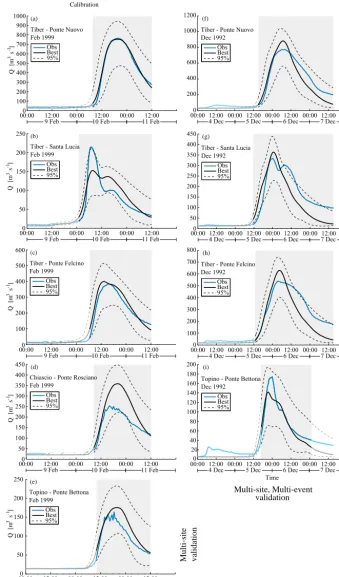
In order to illustrate model performance we selected two major rainfall events within the decade 1990–2000, which generated significant, yet not extreme, floods. The stream-flow triggered by these rainfall events was compared with ob-servational data at the five nodes described in Sect. 3.1. The two events occurred in December 1992 and February 1999. In both cases precipitation was caused by humid frontal ad-vection from the Mediterranean Sea followed by condensa-tion due to orographic uplift (Calenda et al., 2005). For the sake of simplicity, the spatial distribution of the precipita-tion was not retrieved from a climatic model, but was ob-tained by interpolation of the measurements at the available rain gauges (18 and 32 for the events of December 1992 and February 1999, respectively) by means of kriging with exter-nal drift (see, e.g., Goovaerts, 1997). The precipitation was interpolated separately at each time step by using the same exponential semivariogram which has been obtained by an-alyzing offline the available data. In particular, precipitation was first calculated over a 1 km resolution grid and succes-sively aggregated at the macrocell scale, according to the res-olution adopted in the simulations. We remark here that the precipitation data in input can be of any type, the reconstruc-tion by interpolareconstruc-tion with the kriging tool being just a simple example.
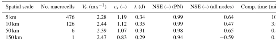
Table 2.Optimal model parameters, calibrated at Ponte Nuovo station (event February 1999), Nash–Sutcliffe efficiency indexes for Ponte Nuovo and all nodes, and computational time cost (for 100 000 runs) resulting from the calibration procedure, for different spatial scale resolutions (size of the macrocell).
Spatial scale No. macrocells Vc(m s−1) cs(–) λ(d) NSE (–) (PN) NSE (–) (all nodes) Comp. time (min)
5 km 476 2.28 1.19 0.34 0.99 0.64 10.2
10 km 126 2.44 1.12 0.35 0.99 0.47 3.00
50 km 6 2.39 1.07 0.31 0.98 0.65 0.44
150 km 1 2.47 0.83 0.29 0.94 −0.59 0.22
1979) with the following boundaries: Vc∈ [0.5,4]m s−1,
cS∈ [0.3,3], andλ∈ [0.01,1]d. The optimization procedure
was based on the maximization of the Nash–Sutcliffe effi-ciency (NSE) index (Nash and Sutcliffe, 1970) for stream-flow evaluated at the outlet of the basin (i.e., Ponte Nuovo, see Fig. 3). The model was run with four spatial resolutions (i.e., 5, 10, 50 and 150 km, see Sect. 3.2) with a computa-tional time step of 1t=0.5h, and calibrated on the event that occurred in the period 6–12 February 1999 at Ponte Nuovo (PN) station. Results in terms of optimized param-eter sets, NSE index, and computational time for the entire set of 100 000 runs are summarized in Table 2.
In all cases, the NSE index at the calibration section (PN) assumes high values, close to one, indicating a very good model fit to the observed streamflow data. Optimal parame-ter sets assume similar values at all the scales, suggesting that the model is able to preserve geomorphological dispersion when the domain is discretized with macrocells of increas-ing dimension. This is verified also when a sincreas-ingle macrocell of 150 km resolution is used, though in this case the impossi-bility to reproduce the spatial variaimpossi-bility of the rainfall (given that only a single macrocell is used the precipitation is con-sidered uniform over the entire basin) resulted in an inaccu-rate description of inter-basin propagation of fluxes, as em-phasized by the negative values of the NSE index averaged over all nodes. Conversely, for all the other spatial resolu-tions, overall NSE values between 0.47 and 0.65 were ob-tained. Notice that all cases with the average NSE>0.45 are with a macrocell dimension equal to or smaller than the inte-gral scale of the precipitation, which is about 36 km (E. Volpi, Modello di struttura spaziale del campo di precipitazione, unpublished technical report, available upon request). It is therefore clear that the inaccuracies encountered with large macrocells are due to the inaccurate spatial description of the precipitation. Finally, the computational cost for 100 000 runs and for a single processor (Intel(R) Xeon(R) W5580 at 3.20 GHz core), the code being written in Fortran 90, is shown to increase from a few seconds in the case of one sin-gle macrocell to about 10 min for the finer resolution (1 km, corresponding to 476 macrocells). We emphasize that the computational efforts can be reduced considerably by imple-menting parallel computing techniques, to which
HYPER-stream is particularly suited thanks to its inherently parallel formulation (see also Sect. 2).
Obs Best 9U4 (a) Tiber[f[Ponte[Nuovo Feb[R999
CC:CC RA:CC CC:CC RA:CC CC:CC RA:CC
9[Feb RC[Feb RR[Feb
ECC ,CC VCC Q [m s ] 3 UCC MCC ICC ACC RCC C 9CC RCCC Obs Best 9U4 Topino[f[Ponte[Bettona Dec[R99A AC C MC EC VC RCC
CC:CC RA:CC CC:CC RA:CC CC:CC RA:CC CC:CC M[Dec U[Dec E[Dec ,[DecRA:CC RAC RMC REC RVC ACC (i) Obs Best 9U4 (b) Tiber[f[Santa[Lucia Feb[R999 RCC UC C RUC ACC AUC
CC:CC RA:CC CC:CC RA:CC CC:CC RA:CC
9[Feb RC[Feb RR[Feb
Obs Best 9U4 Tiber[f[Ponte[Felcino Feb[R999 ECC UCC MCC ICC ACC RCC C
CC:CC RA:CC CC:CC RA:CC CC:CC RA:CC
9[Feb RC[Feb RR[Feb
(c)
Obs Best 9U4
(d)
CC:CC RA:CC CC:CC RA:CC CC:CC RA:CC
9[Feb RC[Feb RR[Feb
C
Obs Best 9U4
(e)
CC:CC RA:CC CC:CC RA:CC CC:CC RA:CC
9[Feb RC[Feb RR[Feb
Time Topino[f[Ponte[Bettona Feb[R999 RCC UC C RUC ACC AUC Obs Best 9U4 (f) Tiber[f[Ponte[Nuovo Dec[R99A
CC:CC RA:CC CC:CC RA:CC CC:CC RA:CC CC:CC M[Dec U[Dec E[Dec ,[DecRA:CC
Obs Best 9U4 Tiber[f[Santa[Lucia Dec[R99A C
CC:CC RA:CC CC:CC RA:CC CC:CC RA:CC CC:CC M[Dec U[Dec E[Dec ,[DecRA:CC
(g)
Obs Best 9U4
C
[image:11.612.128.468.73.651.2]CC:CC RA:CC CC:CC RA:CC CC:CC RA:CC CC:CC M[Dec U[Dec E[Dec ,[DecRA:CC Tiber[f[Ponte[Felcino Dec[R99A (h) Time Chiascio[f[Ponte[Rosciano Feb[R999 Calibration Multi-site, Multi-event validation M ulti-site validation IUC ICC AUC ACC RUC RCC UC MUC MCC RACC RCCC VCC ECC MCC ACC C ECC UCC MCC ICC ACC RCC VCC ,CC IUC ICC AUC ACC RUC RCC UC MUC MCC -1 Q [m s ] 3 -1 Q [m s ] 3 -1 Q [m s ] 3 -1 Q [m s ] 3 -1
83, 59, 100 %, and R factor equal to 1.85, 1.76, 1.50, and 2.37, for PN, PF, SL, and PB, respectively; we note that no water discharge data were available at PR during this event), although a general tendency to underestimate the flood vol-ume is evident. This is likely due to inherent differences between precipitation conditions (e.g., intensity, spatial dis-tribution) during the two events and in the preceding days, which reflect into different initial soil moisture conditions that cannot be fully captured with the simple event-based SCS-CN model used here.
4 Conclusions
This work presents an innovative, multi-scale streamflow routing method based on the travel time approach. The prin-cipal aim is to develop a simple, parsimonious and computa-tionally efficient method for modeling streamflow (and par-ticularly floods) in large basins. The model, coined as HY-PERstream, aims to correctly reproduce the relevant hori-zontal hydrological fluxes across the scales of interest, from a single catchment to the whole continent. The method is based on the WFIUH theory applied to a hybrid raster–vector data structure, which allows the derivation of localized infor-mation on travel times and flow characteristics without the need of narrowing the resolution of the computational grid adopted for the study area. The relevant features of the model are illustrated through the modeling of two flood events in the Upper Tiber river basin (central Italy), with four different do-main discretizations, i.e., different dimensions of macrocells. The main results of the present work can be summarized as follows.
– HYPERstream employs a strategy for modeling cell-scale runoff dispersivity such that the simulation of hor-izontal hydrological fluxes is independent of the grid size, which in turn is a function of the resolution of the atmospheric model or the integral scale of observed precipitation (in case ground-based rainfall measure-ments are used as in the example application provided here). In particular, the contribution of the geomorpho-logical dispersion is kept invariant at all spatial scales, since in our scheme river network response is derived from the morphological information embedded in the available DEM. This “perfect upscaling” characteristic of HYPERstream is particularly important in all cases when the catchment response needs to be accurately represented, e.g., when dealing with extreme events like floods and inundations.
– The above “perfect upscaling” characteristic allows adopting large cells, making the model suitable to large-scale models, up to the continental large-scale. The overall response function of the river networks will anyway be preserved, no matter the discretization.
– Computational efficiency is another relevant feature of the proposed approach. Efficiency stems from the fact that the demanding calculation of the width functions is a pre-processing, one-time effort. Furthermore, the model is prone to parallelization, stemming from the linearity of routing and independency of the runoff gen-eration module adopted at the cell scale. These features make HYPERstream an appealing tool for uncertainty assessment of the predictions, and for simulations con-ducted in a Monte Carlo framework.
– The routing component of the model (including hills-lope routing) depends on two parameters, with the addi-tional parameters inherited from the conceptual model of runoff generation adopted at the hillslope scale. While in principle no limitations are posed to the lat-ter conceptualization, we are in favor of a pragmatic “downward” approach, which limits the total number of parameters, to reduce uncertainty and overparame-terization. Parsimony is important for a meaningful and reliable parameter estimation procedure and uncertainty analysis.
We believe that all of the above characteristics make HY-PERstream an appealing routing tool to be implemented in LHMs, particularly suitable for climate change impact stud-ies where the accuracy of the streamflow routing may be sig-nificantly affected by the spatial resolution adopted.
Acknowledgements. This research has been partially funded by
the Italian Ministry of Public Instruction, University and Research, through the project PRIN 2010–2011 (Innovative methods for water resources management under hydro-climatic uncertainty scenarios, prot. 2010JHF437). S. Piccolroaz, B. Majone, and A. Bellin were also supported by European Union FP7 Collaborative Project GLOBAQUA (Managing the effects of multiple stressors on aquatic ecosystems under water scarcity, grant no. 603629-ENV-2013.6.2.1). Authors also thank the Hydrographic Service of Umbria Region for data provision.
Edited by: R. Moussa
References
Abbaspour, K. C., Faramarzi, M., Ghasemi, S. S., and Yang, H.: As-sessing the impact of climate change on water resources in Iran, Water Resour. Res., 45, W10434, doi:10.1029/2008WR007615, 2009.
Arnell, N. W.: A simple water balance model for the simulation of streamflow over a large geographic domain, J. Hydrol., 217, 314–335, doi:10.1016/S0022-1694(99)00023-2, 1999.
Bellin, A., Majone, B., Cainelli, O., Alberici, D., and Villa, F.: A continuous coupled hydrological and water resources management model, Environ. Modell. Softw., 75, 176–192, doi:10.1016/j.envsoft.2015.10.013, 2016.
Botter, G. and Rinaldo, A.: Scale effect on geomorphologic and kinematic dispersion, Water Resour. Res., 39, SWC61–SWC610, doi:10.1029/2003WR002154, 2003.
Calenda, G., Gorgucci, E., Napolitano, F., Novella, A., and Volpi, E.: Multifractal analysis of radar rainfall fields over the area of Rome, Adv. Geosci., 2, 293–299, doi:10.5194/adgeo-2-293-2005, 2005.
Clark, M. P., Fan, Y., Lawrence, D. M., Adam, J. C., Bolster, D., Gochis, D. J., Hooper, R. P., Kumar, M., Leung, L. R., Mackay, D. S., Maxwell, R. M., Shen, C., Swenson, S. C., and Zeng, X.: Improving the representation of hydrologic processes in Earth System Models, Water Resour. Res., 51, 5929–5956, doi:10.1002/2015WR017096, 2015.
D’Asaro, F. and Grillone, G.: Empirical Investigation of Curve Number Method Parameters in the Mediterranean Area, J. Hydrol. Eng., 17, 1141–1152, doi:10.1061/(ASCE)HE.1943-5584.0000570, 2012.
De Barros, F. P. J. and Rubin, Y.: Modelling of block-scale macrodispersion as a random function, J. Fluid Mech., 676, 514– 545, doi:10.1017/jfm.2011.65, 2011.
De Paiva, R. C. D., Buarque, D. C., Collischonn, W., Bon-net, M. P., Frappart, F., Calmant, S., and Bulhões Mendes, C. A.: Large-scale hydrologic and hydrodynamic modeling of the Amazon River basin, Water Resour. Res., 49, 1226–1243, doi:10.1002/wrcr.20067, 2013.
Di Lazzaro, M.: Regional analysis of storm hydrographs in the Rescaled Width Function framework, J. Hydrol., 373, 352–365, doi:10.1016/j.jhydrol.2009.04.027, 2009.
Di Lazzaro, M. and Volpi, E.: Effects of hillslope dynam-ics and network geometry on the scaling properties of the hydrologic response, Adv. Water Resour., 34, 1496–1507, doi:10.1016/j.advwatres.2011.07.012, 2011.
D’Odorico, P. and Rigon, R.: Hillslope and channel contributions to the hydrologic response, Water Resour. Res., 39, SWC11– SWC19, doi:10.1029/2002WR001708, 2003.
Döll, P., Kaspar, F., and Lehner, B.: A global hydrological model for deriving water availability indicators: Model tuning and validation, J. Hydrol., 270, 105–134, doi:10.1016/S0022-1694(02)00283-4, 2003.
ESRI: ArcGIS Desktop: Release 10, Environmental Systems Re-search Institute, Redlands, CA, USA, available at: http://www. esri.com/software/arcgis/arcgis-for-desktop (last access: 24 Au-gust 2015), 2011.
Freer, J., Beven, K., and Ambroise, B.: Bayesian estimation of un-certainty in runoff prediction and the value of data: An applica-tion of the GLUE approach, Water Resour. Res., 32, 2161–2173, doi:10.1029/95WR03723, 1996.
Giannoni, F., Roth, G., and Rudari, R.: A procedure for drainage network identification from geomorphology and its application to the prediction of the hydrologic response, Adv. Water Resour., 28, 567–581, doi:10.1016/j.advwatres.2004.11.013, 2005.
Gong, L., Widén-Nilsson, E., Halldin, S., and Xu, C. Y.: Large-scale runoff routing with an aggregated network-response function, J. Hydrol., 368, 237–250, doi:10.1016/j.jhydrol.2009.02.007, 2009.
Gong, L., Halldin, S., and Xu, C. Y.: Global-scale river routing-an efficient time-delay algorithm based on HydroSHEDS high-resolution hydrography, Hydrol. Process., 25, 1114–1128, doi:10.1002/hyp.7795, 2011.
Goovaerts, P.: Geostatistics for natural resources evaluation, Uni-versity Press, Oxford, USA, 496 pp., 1997.
Gupta, V. K. and Mesa, O. J.: Runoff generation and hydrologic response via channel network geomorphology - recent progress and open problems, J. Hydrol., 102, 3–28, doi:10.1016/0022-1694(88)90089-3, 1988.
Gupta, V. K., Waymire, E., and Rodríguez-Iturbe, I.: On Scales, Gravity and Network Structure in Basin Runoff, in: Scale Prob-lems in Hydrology, edited by: Gupta, V. K., Rodríguez-Iturbe, I., and Wood, E. F., vol. 6 of Water Science and Technology Library, 159–184, Springer Netherlands, doi:10.1007/978-94-009-4678-1_8, 1986.
Haddeland, I., Clark, D. B., Franssen, W., Ludwig, F., Voß, F., Arnell, N. W., Bertrand, N., Best, M., Folwell, S., Gerten, D., Gomes, S., Gosling, S. N., Hagemann, S., Hanasaki, N., Harding, R., Heinke, J., Kabat, P., Koirala, S., Oki, T., Polcher, J., Stacke, T., Viterbo, P., Weedon, G. P., and Yeh, P.: Multimodel estimate of the global terrestrial water balance: Setup and first results, J. Hydrometeorol., 12, 869–884, doi:10.1175/2011JHM1324.1, 2011.
Hallema, D. W. and Moussa, R.: A model for distributed GIUH-based flow routing on natural and anthropogenic hillslopes, Hy-drol. Process., 28, 4877–4895, doi:10.1002/hyp.9984, 2014. Hallema, D. W., Moussa, R., Andrieux, P., and Voltz, M.:
Param-eterization and multi-criteria calibration of a distributed storm flow model applied to a Mediterranean agricultural catchment, Hydrol. Process., 27, 1379–1398, doi:10.1002/hyp.9268, 2013. Hanasaki, N., Kanae, S., Oki, T., Masuda, K., Motoya, K.,
Shi-rakawa, N., Shen, Y., and Tanaka, K.: An integrated model for the assessment of global water resources – Part 1: Model descrip-tion and input meteorological forcing, Hydrol. Earth Syst. Sci., 12, 1007–1025, doi:10.5194/hess-12-1007-2008, 2008a. Hanasaki, N., Kanae, S., Oki, T., Masuda, K., Motoya, K.,
Shi-rakawa, N., Shen, Y., and Tanaka, K.: An integrated model for the assessment of global water resources – Part 2: Applica-tions and assessments, Hydrol. Earth Syst. Sci., 12, 1027–1037, doi:10.5194/hess-12-1027-2008, 2008b.
Kavvas, M. L., Kure, S., Chen, Z. Q., Ohara, N., and Jang, S.: WEHY-HCM for Modeling Interactive Atmospheric-Hydrologic Processes at Watershed Scale. I: Model Description, J. Hydrol. Eng., 18, 1262–1271, doi:10.1061/(ASCE)HE.1943-5584.0000724, 2013.
Lehner, B. and Grill, G.: Global river hydrography and net-work routing: Baseline data and new approaches to study the world’s large river systems, Hydrol. Process., 27, 2171–2186, doi:10.1002/hyp.9740, 2013.
Lehner, B., Verdin, K., and Jarvis, A.: New global hydrography de-rived from spaceborne elevation data, EOS, Trans. Am. Geophys. Union, 89, 93–94, doi:10.1029/2008EO100001, 2008.
Liang, X., Lettenmaier, D. P., Wood, E. F., and Burges, S. J.: A sim-ple hydrologically based model of land surface water and energy fluxes for general circulation models, J. Geophys. Res.-Atmos, 99, 14415–14428, doi:10.1029/94JD00483, 1994.
Manabe, S.: Climate and the ocean circulation: 1. The atmo-spheric circulation and the hydrology of the Earth’s surface, Mon. Weather Rev., 97, 739–805, 1969.
Manfreda, S., Nardi, F., Samela, C., Grimaldi, S., Taramasso, A. C., Roth, G., and Sole, A.: Investigation on the use of geomorphic approaches for the delineation of flood prone areas, J. Hydrol., 517, 863–876, doi:10.1016/j.jhydrol.2014.06.009, 2014. McKay, M. D., Beckman, R. J., and Conover, W. J.: A Comparison
of Three Methods for Selecting Values of Input Variables in the Analysis of Output from a Computer Code, Technometrics, 21, 239–245, doi:10.2307/1268522, 1979.
Mesa, O. J. and Mifflin, E. R.: On the Relative Role of Hillslope and Network Geometry in Hydrologic Response, in: Scale Problems in Hydrology, edited by Gupta, V. K., Rodríguez-Iturbe, I., and Wood, E. F., vol. 6 of Water Science and Technology Library, 1–17, Springer Netherlands, doi:10.1007/978-94-009-4678-1_1, 1986.
Milly, P. C. D. and Shmakin, A. B.: Global modeling of land water and energy balances. Part I: The land dynamics (LaD) model, J. Hydrometeorol., 3, 283–299, doi:10.1175/1525-7541(2002)003<0283:GMOLWA>2.0.CO;2, 2002.
Montgomery, D. R. and Foufoula-Georgiou, E.: Channel network source representation using digital elevation models, Water Re-sour. Res., 37, 53–71, doi:10.1080/02626669209492561, 1992. Moussa, R.: Geomorphological transfer function calculated from
digital elevation models for distributed hydrological mod-elling, Hydrol. Process., 11, 429–449, doi:10.1002/(SICI)1099-1085(199704)11:5<429::AID-HYP471>3.0.CO;2-J, 1997. Naden, P. S.: Spatial variability in flood estimation for large
catch-ments: the exploitation of channel network structure, 37, 53–71, doi:10.1080/02626669209492561, 1992.
Nash, J. E. and Sutcliffe, J. V.: River flow forecasting through con-ceptual models part I. A discussion of principles, J. Hydrol., 10, 282–290, doi:10.1016/0022-1694(70)90255-6, 1970.
Nazemi, A. and Wheater, H. S.: On inclusion of water resource management in Earth system models – Part 1: Problem definition and representation of water demand, Hydrol. Earth Syst. Sci., 19, 33–61, doi:10.5194/hess-19-33-2015, 2015.
Nicótina, L., Alessi Celegon, E., Rinaldo, A., and Marani, M.: On the impact of rainfall patterns on the hydrologic response, Water Resour. Res., 44, W12434, doi:10.1029/2007WR006654, 2008. Niu, G. Y., Yang, Z. L., Mitchell, K. E., Chen, F., Ek, M. B., Barlage,
M., Kumar, A., Manning, K., Niyogi, D., Rosero, E., Tewari, M., and Xia, Y.: The community Noah land surface model with multiparameterization options (Noah-MP): 1. Model description and evaluation with local-scale measurements, J. Geophys. Res.-Atmos., 116, D12204, doi:10.1029/2010JD015139, 2011. O’Callaghan, J. F. and Mark, D. M.: The extraction of drainage
net-works from digital elevation data., Comput. Vision Graph., 28, 323–344, 1984.
Oleson, K., Lawrence, D. M., Bonan, G. B., Drewniak, B., Huang, M., Koven, C. D., Levis, S., Li, F., Riley, W. J., Subin, Z. M.,
Swenson, S., Thornton, P. E., Bozbiyik, A., Fisher, R., Heald, C. L., Kluzek, E., Lamarque, J. F., Lawrence, P. J., Leung, L. R., Lipscomb, W., Muszala, S. P., Ricciuto, D. M., Sacks, W. J., Sun, Y., Tang, J., and Yang, Z. L.: Technical description of version 4.5 of the Community Land Model (CLM). NCAR Technical Note NCAR/TN-503+STR, Tech. rep., National Center for At-mospheric Research, doi:10.5065/D6RR1W7M, 2013.
Pilgrim, D. H.: Travel times and nonlinearity of flood runoff from tracer measurements on a small watershed, Water Resour. Res., 12, 487–496, doi:10.1029/WR012i003p00487, 1976.
Pilgrim, D. H.: Isochrones of travel time and distribution of flood storage from a tracer study on a small watershed, Water Resour. Res., 13, 587–595, doi:10.1029/WR013i003p00587, 1977. Prentice, I. C., Liang, X., Medlyn, B. E., and Wang, Y.-P.:
Re-liable, robust and realistic: the three R’s of next-generation land-surface modelling, Atmos. Chem. Phys., 15, 5987–6005, doi:10.5194/acp-15-5987-2015, 2015.
Rigon, R., Bancheri, M., Formetta, G., and de Lavenne, A.: The ge-omorphic unit hydrograph from a historical-critical perspective, Earth Surf. Proc. Land., 41, 27–37, doi:10.1002/esp.3855, 2015.
Rinaldo, A., Marani, A., and Rigon, R.:
Geomorpho-logical dispersion, Water Resour. Res., 27, 513–525,
doi:10.1029/90WR02501, 1991.
Rinaldo, A., Vogel, G. K., Rigon, R., and Rodriguez-Iturbe, I.: Can One Gauge the Shape of a Basin?, Water Resour. Res., 31, 1119– 1127, doi:10.1029/94WR03290, 1995.
Rinaldo, A., Botter, G., Bertuzzo, E., Uccelli, A., Settin, T., and Marani, M.: Transport at basin scales: 1. Theoretical frame-work, Hydrol. Earth Syst. Sci., 10, 19–29, doi:10.5194/hess-10-19-2006, 2006.
Rodríguez-Iturbe, I. and Rinaldo, A.: Fractal river basins: Chance and self-organization, Cambridge University Press, Cambridge, UK, 547 pp., 1997.
Rubin, Y., Sun, A., Maxwell, R., and Bellin, A.: The concept of block-effective macrodispersivity and a unified approach for grid-scale- and plume-scale-dependent transport, J. Fluid Mech., 395, 161–180, doi:10.1017/S0022112099005868, 1999. Samaniego, L., Kumar, R., and Attinger, S.: Multiscale
pa-rameter regionalization of a grid-based hydrologic model
at the mesoscale, Water Resour. Res., 46, W05301,
doi:10.1029/2008WR007327, 2010.
Sapriza-Azuri, G., Jódar, J., Navarro, V., Slooten, L. J., Carrera, J., and Gupta, H. V.: Impacts of rainfall spatial variability on hydrogeological response, Water Resour. Res., 51, 1300–1314, doi:10.1002/2014WR016168, 2015.
Sivapalan, M.: Process complexity at hillslope scale, process sim-plicity at the watershed scale: is there a connection?, Hydrol. Pro-cess., 17, 1037–1041, doi:10.1002/hyp.5109, 2003.
Tarboton, D. G., Bras, R. L., and Rodrìguez-Iturbe, I.: On the ex-traction of channel networks from digital elevation data, Hydrol. Process., 5, 81–100, doi:10.1002/hyp.3360050107, 1991. U.S. Soil Conservation Service: SCS National Engineering
Hand-book, vol. Hydrology, Section 4, US Department of Agriculture, Washington DC, 1964.
Van Beek, L. P. H., Wada, Y., and Bierkens, M. F. P.: Global monthly water stress: 1. Water balance and water availability, Water Re-sour. Res., 47, W07517, doi:10.1029/2010WR009791, 2011. van der Knijff, J. M., Younis, J., and de Roo, A. P. J.: LISFLOOD:
bal-ance and flood simulation, Int. J. Geogr. Inf. Sci., 24, 189–212, doi:10.1080/13658810802549154, 2010.
Van Der Tak, L. D. and Bras, R. L.: Incorporating hillslope effects into the geomorphologic instantaneous unit hydrograph, Water Resour. Res., 26, 2393–2400, doi:10.1029/90WR00862, 1990. Verzano, K., Bärlund, I., Flörke, M., Lehner, B., Kynast, E.,
Voß, F., and Alcamo, J.: Modeling variable river flow ve-locity on continental scale: Current situation and climate change impacts in Europe, J. Hydrol., 424–425, 238–251, doi:10.1016/j.jhydrol.2012.01.005, 2012.
Volpi, E., Di Lazzaro, M., and Fiori, A.: A simplified frame-work for assessing the impact of rainfall spatial variability on the hydrologic response, Adv. Water Resour., 46, 1–10, doi:10.1016/j.advwatres.2012.04.011, 2012.
Vörösmarty, C. J., Federer, C. A., and Schloss, A. L.: Potential evaporation functions compared on US watersheds: Possible im-plications for global-scale water balance and terrestrial ecosys-tem modeling, J. Hydrol., 207, 147–169, doi:10.1016/S0022-1694(98)00109-7, 1998.
Wen, Z., Liang, X., and Yang, S.: A new multiscale routing frame-work and its evaluation for land surface modeling applications, Water Resour. Res., 48, W08528, doi:10.1029/2011WR011337, 2012.
Whiteaker, T. L., Maidment, D. R., Goodall, J. L., and Taka-matsu, M.: Integrating arc hydro features with a schematic
network, Trans. GIS, 10, 219–237,
doi:10.1111/j.1467-9671.2006.00254.x, 2006.
Widén-Nilsson, E., Halldin, S., and Xu, C. y.: Global
water-balance modelling with WASMOD-M: Parameter
es-timation and regionalisation, J. Hydrol., 340, 105–118, doi:10.1016/j.jhydrol.2007.04.002, 2007.
Wood, E. F., Roundy, J. K., Troy, T. J., van Beek, L. P. H., Bierkens, M. F. P., Blyth, E., de Roo, A., Doell, P., Ek, M., Famiglietti, J., Gochis, D., van de Giesen, N., Houser, P., Jaffe, P. R., Kol-let, S., Lehner, B., Lettenmaier, D. P., Peters-Lidard, C., Siva-palan, M., Sheffield, J., Wade, A., and Whitehead, P.: Hyperres-olution global land surface modeling: Meeting a grand challenge for monitoring Earth’s terrestrial water, Water Resour. Res., 47, W05301, doi:10.1029/2010WR010090, 2011.