Star based a Posteriori Error Estimator for Convection Diffusion Problems

Star-based a Posteriori Error Estimator for

Convection Diffusion Problems

B. Achchab

1

,

A. Agouzal

2,∗

,

N. Debit

2

,

K. Bouihat

1

1_{Universit´e Hassan 1}er_{, LM}2_{CE et LAMSAD, FSEJSS et ESTB, B.P 218 Berrechid, Maroc} 2_{Universit´e de Lyon; CNRS ; Universit´e Lyon 1 ; Institut Camille Jordan,}

Bˆatiment Jean Braconnier 21, Avenue Claude Bernard 69622 Villeurbanne cedex,France

∗_{Corresponding Author: [email protected]}

Copyright c⃝2014 Horizon Research Publishing All rights reserved.

Abstract

In this paper, we derive an a posteriori error estimator, for nonconforming finite element approxi-mation of convection-diffusion equation. The a posteriori error estimator is based on the local problems on stars. Finally, we prove the reliability and the efficiency of the estimator without saturation assumption nor comparison with residual estimator

Keywords

A posteriori error estimator, nonconforming finite elements method, convection diffusion equations

AMS subject classification: 65D05, 65D15, 65N50

1

Introduction

A posteriori error estimators provide the basis for adaptive mesh refinement and quantitative error control [1, 8, 4, 5, 12, 19, 14, 10]. One of the most successful estimators was proposed by Bank and Weiser and extended by many authors [2, 3, 7, 13, 16, 20, 21], it is based on the solution of local Neumann problems on elements, which seem to allow for cancelation and thus lead to better results than the residual estimators. The classical proof of equivalence with the energy error require the saturation assumption : this says that the solution can be approximated asymptotically better with quadratic than with linear finite elements. The saturation assumption is shown to be superfluous by Nochetto in [17]. However, removing this assumption requires comparison with residual estimators. More recently, a new a posteriori error estimators on stars was proposed in [15], and the proof of the equivalence with energy error it applies directly without reference to residual estimators.

In this paper, we extended the results of [15] to the case of nonconforming finite elements and the convection diffusion case. A new a posteriori error estimator is introduced based on the solution of a small discrete problem in stars. We prove the reliability and the efficiency of the estimator without saturation assumption nor comparison with residual estimator. We consider the simpler case of nonconforming approximations for convection diffusion problem, and we introduced a technique which allowed us to define a new a posteriori error estimator which are equivalent to the energy error.

2

Setting the problem

We consider here the convection-diffusion problem:

(P)

  

−ε∆u+β.∇u=f in Ω, u= 0 on Γ =∂Ω

In the following we assume that Ω∈R2 _{a simply connected polygon domain, 0< ε <<1 ,β ∈(W}1,∞_(Ω))2_,,

such that−1₂divβ≥a >0 andf ∈L2(Ω). LetTh be a family of conforming shape-regular triangulation of Ω by

lowest order non-conforming Crouzeix-Raviart finite element space defined by:

Vh = {vh∈L2(Ω);∀T ∈ Th, vh_|T ∈P1(T),

∀E∈EI,

∫

E

[vh]Edσ= 0 and∀E ∈Ef,

∫

E

vhdσ= 0}.

where [.]E denoted the jump of the function acrossE. For eachT ∈ Th,we denote by Pk(T) the polynomial space

of degree less than or equal tok.

For all T ∈ Th, we define ∂T− such the part of the frontier ofT such thatβ.nT <0 wherenT stands for the

unit outward normal vector toT on∂T.

In the sequel, we consider uN C_h ∈Vh be a solution of the stabilized nonconforming approximation problem:

(Ph)N C

          

∀vh∈Vh,

∑

T_∈Th

∫

T

[ε∇uN C_h .∇vh+β.∇uN Ch vh]dx

+1₂∑_T∈Th∫_∂T−β.n[uN Ch ]vhdσ=

∫

Ω

f vhdx.

2.0.1 The a posteriori error estimator

For the a posteriori error analysis of the considered approximation, we need to define some local spaces and problems. We denoted by {xi}i_∈N the set of all nodes of the triangulation Th. For each i∈ N, ϕi denoted the

canonical continuous piecewise linear basis function corresponding to xi. The star ωi is the interior relative to Ω

of the support ofϕi, andhi is the maximal size of the elements formingωi. Finally, Γiwill denote the union of the

sides touchingxi that are contained in Ω, and Γiwill denote the union of the sides touchingxithat are contained

in Ω.

For each starωi,i∈ N, ifxi we introduce the spaceV(ωi) defined by

V(ωi) ={v∈Hloc1 (ωi) :

∫

ωi

vϕidx= 0},

if xi is an interior node,

and

V(ωi) ={v∈Hloc1 (ωi) :v= 0 on∂ωi∩Γ},

if xi is a boundary node.

We have the following result of ([15])

Proposition 1 There exists a constant C, only depending on the minimum angle of the triangulation but inde-pendent of the star being considered, such that:

∀v∈V(ωi) ∥v∥0,ωi ≤Chi(

∫

ωi

|∇v|2ϕidx)1/2. (1)

We define the finite dimensional local spaces P2

0(ωi) as follows,

Definition 2 For i∈ N, letP2_(ω

i)denote the space of continuous piecewise quadratic functions on star ωi that vanish on∂ωi. The spacesP02(ωi)is defined byP02(ωi) =P2(ωi)∩V(ωi).

In the following we consider the energy norm:

||u||2_ε,ωi =ε∥∇u∥2_0,ω

i+∥u∥

2 0,ωi.

LetuN C

h ∈Vh be fixed and we denoted by∇huh

the vector belonging to (L2_(Ω))2 _{defined by}

For each i∈ N, we consider the local problems :

(P1)i

              

Findηi∈ P02(ωi) such that ∀µi∈ P02(ωi)

∫

ωi

(ε∇ηi.∇µi)ϕidx=

∫

ωi

(ε∇huN Ch .∇µi)ϕidx

+∫_ω

i(β.∇hu N C

h µi)ϕidx

+1 2

∑

T∈Th

∫

∂T−

β.n[uN C_h ]µiϕidσ−

∫

ωi

f µiϕidx.

and

(P2)i

  

Findαi∈ P02(ωi) such that∀µi∈ P02(ωi)

∫

ωi

(ε∇αi.∇µi)ϕidx=

∫

ωi

ε∇huN Ch .Curl (µiϕi)dx.

Using Lax-Milgram theorem, we prove that the discrete problems have unique solution. The problems (P1)i

estimate the approximation error, but the problems (P2)i estimate the consistency error of the used method.

Finally we set:

∀i∈ N, E21,i(uN Ch ) =

∫

ωi

ε|∇ηi|2ϕidx,

and

∀i∈ N, E2_2,i(uN C_h ) =

∫

ωi

ε|∇αi|2ϕidx.

2.0.2 Upper bound of the error

In this section we prove the one of main results of this paper. First, we prove the upper bound of the error without oscillation. As in ([6],[9],[11]). Recall that [18]:

Lemma 3 (Discrete Poincar and Friedrichs inequalities ).

There is a positives constantsC depending only on the minimum angle ofTh the Ωsuch that:

∀v∈H₀1(Ω) +Vh, ∥v∥20,Ω≤C(

∑

T∈Th

∥∇v∥2_0,Ω). (2)

We have the following global upper bond of the error:

Theorem 4 LetuN C

h ∈Vhsuch that(Ph)N Cholds. There is a positive constantC1depending only on the minimum

angle ofTh such that

∥u−uN C_h ∥ε,Ω ≤ C1[(

∑

i∈N

(E₁2_,i(uN C_h ) +E₂2_,i(uN C_h )))12

+ ∥β∥1,∞hi(

∑

i∈N

E22,i(uN Ch ))

1 2_,

+ ∑

i_∈N

(hi

∑

T_⊂ωi

∥[uN C_h ]∥L2_(∂T)

+ (∥β∥0,∞+∥β∥H(div,ωi))hi∥u N C h ∥0,ωi)

+ osc(f)]. (3)

whereosc(f) is the data oscillations defined by: osc(f) = (∑

i∈N

α2i∥(f−fi)ϕ

1 2

i ∥0,ωi)

1 2_.

where fi=

∫

ωif ϕidx

∫

ωiϕidx

and αi=min(1,√hi_ε).

Proof. Remark that using Helmholtz-decomposition, we have

∇huN Ch − ∇u=∇w+ Curlζ, (4)

withw∈H1

0(Ω),ζ∈H1(Ω) and

∫

Ω

∇w.Curlζdx= 0.

Let us remark also that the orthogonality implies the following error decomposition :

ε∥∇huN Ch − ∇u∥20,Ω=ε∥∇w∥20,Ω+ε∥Curlζ∥20,Ω.

and the following equalities :

ε∥∇w∥2_Ω=

∫

Ω

and

ε∥Curlζ∥2_0,Ω=

∫

Ω

ε(∇huN Ch − ∇u).Curlζdx. (6)

The estimates of expressions in (5) and (6) will be established respectively in the Lemmas 7 and 8 . As a main tool we use the following Lemmas.

Lemma 5 For each node i∈ N there exists an unique operator

Πi:V(ωi)−→ P02(ωi), such that for anyv∈V(ωi) the following conditions hold : 1. For all edge E⊂Γi,

∫

E

(v−Πiv)ϕidσ= 0.

2.

∫

ωi

(v−Πiv)ϕidx= 0

3. ε(

∫

ωi

|∇Πiv|2ϕi)

1 2 _{+ (}

∫

ωi

|Πiv|2ϕi)

1 2 ≤_C

[

ε(

∫

ωi

|∇v|2ϕi)

1 2 ₊

∫

ωi

|v|2ϕi)

1 2

]

,

4. (∑

i_∈N

α−_i2∥(v−Πi(v))(ϕi)

1 2∥2

0,ωi)

1

2 ≤C∥v∥_ε,Ω

where the constant C depends only on the minimum angles ofTh.

The Lemma 5, is an adaptation of arguments given in [15], and so the proof will be skipped.

Lemma 6 For each node i∈ N,Πi defined in the 5, functionsv∈V(ωi),ζ∈V(ωi) anduN Ch ∈Vh. We have

∫

ωi

ε∇huN Ch .∇((Πiv)ϕi)dx=

∫

ωi

ε∇huN Ch .∇(vϕi)dx, (7)

and ∫

ωi

ε∇huN Ch .Curl ((Πiζ)ϕi)dx=

∫

ωi

ε∇huN Ch .∇(ζϕi)dx. (8)

Proof. If we denoted by [∂u

N C h

∂nE

]∈P0(E) the jump of the normal derivative across the edge E. By Green formula

and by lemma 5, we have _∫

ωi

ε∇huN Ch .∇((Πiv)ϕi)dx

=∑_E⊂ω

i

∫

Eε[ ∂uN C

h

∂nE ](Πiv)ϕidx

= ∑

E⊂ωi

∫

E

ε[∂u

N C h

∂nE

]vϕidx=

∫

ωi

ε∇huN Ch .∇(vϕi)dx.

To prove the second equality, if we denoted by [∂uN Ch

∂τE ]∈P0(E) the jump of the tangential derivative across the edge E. We have by Green formula and lemma 5

∫

ωi

ε∇huN Ch .Curl ((Πiζ)ϕi)dx=

∑

E_⊂ωi

∫

E

ε[∂u

N C h

∂τE

](Πiζ)ϕidx

= ∑

E⊂ωi

∫

E

ε[∂u

N C h

∂τE

]ζϕidx=

∫

ωi

ε∇huN Ch .Curl (ζϕi)dx.

The following Lemma give an estimate of expression (5):

Lemma 7 For w ∈ H1

0(Ω) defined in (4), there exists positives constants C∗, depending only on the minimum

angle of Th such that

∥w∥ε,Ω ≤ C∗[(

∑

i_∈N

(E₁2_,i(uN C_h )))12

+ ∥β∥1,∞hi(

∑

i∈N

E2_2,i(uN C_h ))12,

+ ∑

i∈N

(hi

∑

T⊂ωi

∥[uN C_h ]∥L2_(∂T)+ (∥β∥0,_∞

+ ∥β∥H(div,ωi))hi∥u N C h ∥0,ωi),

Proof . Forw∈H1

0(Ω) defined in (4), we set

wh=

∑

i∈N

wiϕi, wherewi=

∫

ωiwϕidx

∫

ωiϕidx

for interior nodes, andwi= 0 otherwise.

By adapting standard arguments used in the analysis of finite element approximation, and by using the propriety

−1

2divβ≥a >0, wa have:

a∥w∥2ε,Ω ≤

∫

Ω

ε∇w.∇w

+

∫

Ω

β.∇wwdx,

where: ε∥∇w∥2_Ω=∫_Ωε(∇huN Ch − ∇u).∇wdx and

∫

Ω

∇w.Curlζdx= 0. This gives,

∫

Ω

ε∇w.∇w+

∫

Ω

β.∇ww =

∫

Ω

ε∇w.(∇huN Ch − ∇u)dx

+

∫

Ω

β.(∇huN Ch − ∇u)w

−

∫

Ω

β.wCurlζdx

−

∫

Ω

ε.∇w.Curlζdx

=

∫

Ω

ε∇huN Ch .∇wdx

+

∫

Ω

β.∇huN Ch wdx

−

∫

Ω

ε∇u.∇wdx−

∫

Ω

β.∇uwdx

−

∫

Ω

β.wCurlζdx

−

∫

Ω

ε.∇w.Curlζdx.

Sincewh∈Vh∩H01(Ω), a(w, wh) = 0, we have: a(w, w) =a(w, w−wh). Then

a∥w∥2_ε,Ω ≤

∫

Ω

ε∇huN Ch .∇(w−wh)dx

+

∫

Ω

β.∇huN Ch (w−wh)dx

−

∫

Ω

ε∇u.∇(w−wh)dx−

∫

Ω

β.∇u(w−wh)dx

−

∫

Ω

β.(w−wh)Curlζdx.

Stating that

w−wh=

∑

i∈N

(w−wi)ϕi, and using

∑

i∈N

ϕi= 1 gives

a∥w∥2_ε,Ω ≤ ∑

i_∈N

[

∫

ωi

ε∇huN Ch .∇(w−wi)ϕidx

+

∫

ωi

β.∇huN Ch (w−wi)ϕidx]

− ∑

i∈N

[

∫

ωi

f(w−wi)ϕidx

−

∫

ωi

Since (w−wi)∈V(ωi), adding and removing same quantities in the two last terms give:

a∥w∥2_ε,Ω

≤∑

i_∈N

[

∫

ωi

ε∇huN Ch .∇Πi(w−wi)ϕi)dx

+

∫

ωi

β.∇huN Ch Πi(w−wi)ϕidx]

+∑

i_∈N

[1 2

∑

T_⊂ωi

∫

∂T−

|β.n|[uN C_h ](Πi(w−wi))ϕidσ]

−∑

i∈N

[

∫

ωi

fΠi(w−wi)ϕidx]

−∑

i∈N

[1 2

∑

T⊂ωi

∫

∂T−

|β.n|[uN C_h ](Πi(w−wi))ϕidσ]

+∑

i_∈N

[

∫

ωi

β.∇huN Ch (w−wi−Πi(w−wi))ϕidx]

−∑

i∈N

[

∫

ωi

f(w−wi−Πi(w−wi))ϕidx]

+ [

∫

ωi

β.(w−wi)ϕiCurlζdx].

Using the definition of local problems (P1)i,

a∥w∥2_ε,Ω

≤∑

i∈N

[

∫

ωi

ε∇ηi.∇Πi(w−wi)ϕi)dx]

−∑

i∈N

[

∫

ωi

f(w−wi−Πi(w−wi))ϕidx]

−∑

i∈N

[1 2

∑

T⊂ωi

∫

∂T−

|β.n|[uN C_h ](Πi(w−wi))ϕidσ]

+ [∑

i_∈N

∫

ωi

β.∇huN Ch (w−wi−Πi(w−wi))ϕidx]

−∑

i∈N

[

∫

ωi

β.(w−wi)ϕiCurlζdx].

We now process successively with each term of the right-hand side. On one hand, using Cauchy-Schwarz and item 3 of lemma 5 we have:

∫

ωi

ε∇ηi.∇Πi(w−wi)ϕidx

≤( ∑

i_∈N

∫

ωi

ε|∇ηi|2ϕidx

)1

2( ∑

i_∈N

∫

ωi

ε|∇Πi(w−wi)|2ϕidx

)1 2

,

≤C( ∑

i∈N

E₁2_,i(uN C_h )

)1

2( ∑

i∈N

∫

ωi

ε|∇(w−wi)|2ϕidx

)1 2

,

≤C( ∑

i_∈N

E₁2_,i(uN C_h )

)1 2

∥w∥ε,Ω.

On the other hand, since both of (w−wi) and Πi(w−wi) belong toV(wi), using definition ofV(wi) and coefficients

fi give:

∑

i_∈N

[∫

ωi

f(w−wi−Πi(w−wi))ϕidx

]

=∑

i∈N

[∫

ωi

(f−fi)(w−wi−Πi(w−wi))ϕidx

Using Cauchy-Schwarz, the proposition 1, the item 4 of lemma 5 and once more ∑

i∈N

ϕi= 1 we get

∑

i∈N

[∫

ωi

f(w−wi−Πi(w−wi))ϕidx

]

≤osc(f)(∑

i_∈N

α−_i 2∥(w−wi−Πi(w−wi))(ϕi)

1 2∥2

0,ωi)

1 2_, ≤C osc(f)∥w∥ε,Ω.

C is a generic constant only depending on the minimum angle of triangulation. We note:

A = ∑

i∈N

[∫

ωi

β.∇huN Ch (w−wi−Πi(w−wi))ϕidx

] − [ 1 2 ∑

T⊂ωi

∫

∂T−

|β.n|[uN C_h ](Πi(w−wi))ϕidσ

]

Using the Green formula we have:

A=∑

i∈N

[∫

ωi

β.∇huN Ch (w−wi−Πi(w−wi))ϕidx

] − [ 1 2 ∑

T_⊂ωi

∫

∂T−

|β.n|[uN C_h ](Πi(w−wi))ϕidσ

] =∑ i_∈N [ 1 2 ∑ T_∈Th ∫ ∂T−

|β.n|[uN C_h ](w−wi−Πi(w−wi))ϕidσ

]

−∑

i∈N

[∫

ωi

β.uN C_h ∇(w−wi−Πi(w−wi))ϕidx

]

+∑

i∈N

[∫

ωi

divβ.uN C_h (w−wi−Πi(w−wi))ϕidx

] − [ 1 2 ∑

T⊂ωi

∫

∂T−

|β.n|[uN C_h ](Πi(w−wi))ϕidσ

]

.

Using Cauchy-Schwarz and the proposition 1 we have:

A = ∑

i∈N

[

∫

ωi

β.∇huN Ch (w−wi−Πi(w−wi))ϕidx]

− [1 2

∑

T_⊂ωi

∫

∂T−

|β.n|[uN C_h ](Πi(w−wi))ϕi]

≤ C[∑

i∈N

(hi

∑

T⊂ωi

∥[uN C_h ]∥L2_(∂T)+ (∥β∥0,_∞

+ ∥β∥H(div,ωi))hi∥u N C

h ∥0,ωi) +osc(f)].

Finally: ∑ i∈N [ ∫ ωi

β.(w−wi)Curlζdx]

≤ ∥β∥1,∞∥Curlζ∥0,ω∥(w−wi)∥0,ω

≤C∥β∥1,∞(

∑

i∈N

E₍₂2_,i)(uN C_h ))12∥_w∥_ε,ω

i.

Summing up the different contributions in the estimate of∥w∥ε,ωi and using the continuity ofa(., .) yield the result.

We have also the following result giving an estimation of expression (6):

Lemma 8 Forζ∈H1_{(Ωdefined in (4), there exists a positive constant C, depending only on the minimum angle}

ofTh such that

ε12∥Curlζ∥_0,Ω≤C(

∑

i∈N

Proof. Letζ∈H1_{(Ω) defined in (4), we note}

ζh=

∑

i∈N

ζiϕ, whereζi=

∫

ωiζϕidx

∫

ωiϕidx

for all nodes. First, using (6) and the fact that _∫

Ω

ε∇w.Curlζdx= 0.

Which easy to verify that:

ε∥Curlζ∥2_0,Ω =

∫

Ω

ε(∇huN Ch − ∇u).Curlζdx

=

∫

Ω

ε∇huN Ch .Curlζdx,

and hence:

ε∥Curlζ∥20,Ω =

∫

Ω

ε∇huN Ch .Curl (ζ−ζh)dx

+

∫

Ω

ε∇huN Ch .Curlζhdx.

On one hand, since: Curlζh ∈ H(div ; Ω), div(Curlζh) = 0, and ∀T ∈ Th, (Curlζh)_|T belonging the lowest

Raviart-Thomas spaceRT0(T) = (P0(T))2+xP0(T) anduN Ch ∈Vh, by Green formula we have

∫

Ω

∇huN Ch .Curlζhdx= 0.

On the other hand, since (ζ−ζi)∈V(ωi), using Lemma 5, and the definition of local problem (P2)i we have, for

alli∈ N :

∑

i_∈N

[∫

ωi

ε∇huN Ch Curl ((ζ−ζi)ϕi)dx

]

=∑

i_∈N

[∫

ωi

ε∇huN Ch Curl (Πi(ζ−ζi)ϕi)dx

]

=∑

i∈N

[∫

ωi

ε(∇αi.∇Πi(ζ−ζi))ϕidx

]

.

Using the last equalities, ∑

i∈N

ϕi = 1 and the equality∥Curlζ∥0,Ω=∥∇ζ∥0,Ω , we obtain

ε∥Curlζ∥2_0,Ω

=∑

i_∈N

∫

ωi

ε(∇huN Ch .Curl (ζ−ζh))ϕidx

=∑

i∈N

∫

ωi

ε(∇huN Ch .Curl (Πi(ζ−ζh)))ϕidx

=∑

i_∈N

∫

ωi

ε∇αi.∇(Πi(ζ−ζh))ϕidx

≤C(∑

i∈N

E₍₂2_,i)(uN C_h ))12₍

∑

i∈N

∫

ωi

ε|∇ζ|2ϕidx)

1 2

≤C(∑

i_∈N

E₍₂2_,i)(uN Ch ))

1

2_ε12∥_Curlζ∥_0,Ω.

Which completes proof of the lemma.

The combination of the two lemmas 7 and 8, gives the result of the upper bound of the error of the theorem 4.

2.0.3 Lower bound of the error

In this section we prove a lower bound of the error without oscillation.

Theorem 9 Let uN C

h ∈Vh, there exists a positives constants C1 andC2, depending on the minimum angle of the

triangulation such that, for any i∈ N,

and

E2,i(uN Ch )≤C2||u−uN Ch ||ε,wi. Proof. Leti∈ N. We have

E₁2_,i(uN C_h ) =

∫

ωi

(ε∇huN Ch .∇ηi)ϕidx+

∫

ωi

(β.∇huN Ch ηi)ϕidx

−

∫

ωi

f ηiϕidx+

1 2

∑

T_⊂ωi

∫

∂T−

|β.n|[uN C_h ]ηiϕidσ.

Then

E₍₁2_,i)(uh) =

∫

ωi

(ε∇huN Ch .∇ηi)ϕidx+

∫

ωi

(β.∇huN Ch ηi)ϕidx

−

∫

ωi

f ηiϕidx

+ 1

2

∑

T_⊂ωi

∫

∂T−

|β.n|[uN Ch ]ηiϕidσ,

=

∫

ωi

(ε(∇huN Ch − ∇u).∇(ηiϕi)dx

+

∫

ωi

(β.(∇huN Ch − ∇u)ηi)ϕidx

+ 1

2

∑

T⊂ωi

∫

∂T−

|β.n|[uN Ch ]ηiϕidσ,

=

∫

ωi

(ε(∇huN Ch − ∇u).∇(ηi)ϕidx

+

∫

ωi

(ε(∇huN Ch − ∇u).∇(ϕi)ηidx

+

∫

ωi

(β.(∇huN Ch − ∇u)ηi)ϕidx

+ 1

2

∑

T⊂ωi

∫

∂T−

|β.n|[uN C_h ]ηiϕidσ.

Using Cauchy-Schwarz theorem imply that:

E₍₁2_,i)(uN C_h ) ≤ ε12∥∇u− ∇_huN C

h ∥0,ωi(ε

∫

ωi

|∇ηi|2ϕidx)

1 2

+ ε12∥∇u− ∇_huN C

h ∥0,ωiε

1 2∥η_i∥_0,ω

i∥ϕi∥1,∞,ωi

+ ∥β∥0,_∞∥∇u− ∇huN Ch ∥0,ωi(

∫

ωi

|ηi|2ϕidx)

1 2

+ C∥[uN C_h ]∥L2_(∂T)∥η_i∥_0,ωi.

Or:

ε12∥η_i∥₀≤C h_iε 1 2(

∫

ωi

(|∇ηi|2ϕidx)))

1 2.

Then

ε12∥_ηi∥_0,ω

i ≤C hiE(1,i)(u N C h ).

and sinceηi∈V(ωi), we have |ϕi|1,_∞,ωi ≤

C hi

. And:

∑

T∈Th

∫

∂T−

|β.n|[uN C_h ]ηiϕidσ

≤C∥[uN C_h ]∥L2_(∂T)∥η_i∥_0,ωi ≤Cε−41α

1 2

T∥[u N C

h ]∥L2_(∂T)E_1,i(uN C_h ) ≤C||u−uN C_h ||ε,wiE1,i(u

Summing up the different contributions in the estimate ofE1,i(uN Ch ) we get:

E1,i(uN Ch )≤C(1 +∥β∥1,∞hi)||u−uN Ch ||ε,wi.

To prove the second inequality, let us remark that, using Green formula, we have :

∀µi∈ P02(ωi);

∫

ωi

ε∇u.Curl (µiϕi)dx= 0.

Then using Cauchy-Schwartz inequality we deduce

E2_(2,i)(uN C_h ) =

∫

ωi

ε∇huN Ch .Curl (αiϕi)dx

=

∫

ωi

ε(∇huN Ch − ∇u).Curl (αiϕi)dx

≤ ε12||∇_u− ∇_uN C

h ||0,wiε

1

2||_{Curl (αiϕi)}||_0,w

i.

Where

ε12||Curl (α_iϕ_i)||_0,w

i ≤CE(2,i)(u N C h ).

Then

E(2,i)(uN Ch )≤Cε

1

2||∇u− ∇uN C

h ||0,wi ≤C||u−u N C h ||ε,wi

3

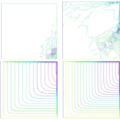
Mesh adaption procedure and Numerical results

Example 1. We now consider, on the same domain Ω =]0,1[×]0,1[, the convection diffusion reaction problem:

−ϵ∆u+β.∇u=f.

withu= 0 on∂Ω such thatβ = [3,2]t,ϵ= 0.01, and f = 1

This solution, for smallϵ >0, exhibits boundary layers near the top (y= 1) and right (x= 1) boundaries. The adaptive finite element method correctly refines in these layers, yielding accurate solutions with a small number of unknowns (relative to uniform refinement). The meshes and the contour maps are omitted for brevity reasons (see Fig 1 and Fig 2).

[image:10.595.201.404.483.682.2]

The interesting point of this problem concerns the exactness of estimators as ϵgoes to zero

[image:11.595.189.389.52.253.2] [image:11.595.187.394.290.464.2]

Figure 2. The isovalus of the solution .

Figure 3. Decay of error indicator. The dashed line has slope of−1₂.

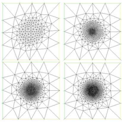
Example 2. We now consider, on the same domain Ω =]0,1[×]0,1[, the convection diffusion reaction problem:

−ϵ∆u+β.∇u=f.

With the source termf given by the exact solution,

u=xy(x−1)(y−1)e−100(x−0.5)2−100(y−0.5)2

which presents sharp curvature in the vicinity of point (0.5,0.5), and we perform a nonconforming finite element discretization on it. Successive iterations of adaptive mesh are represented in Figure 4. Computed and Exact solution are given in Figure 5, where the scaling of the height is the same for both pictures.

Remarks.

1. We can write a general framework regroups the conforming and nonconforming approximations of the con-vection diffusion problem, just write the approximate problem as:

(Ph)

          

F ind uh∈Wh, such that: ∀vh∈Wh,

∑

T_∈Th

∫

T

[ε∇uh.∇vh

+β.∇uhvh]dx+1₂

∑

T_∈Th

∫

∂T−β.n[uh]vhdσ

=∫_Ωf vhdx.

withWh=Vh∩H01(Ω)) in the conforming case andWh=Vhin the non conforming case. The same arguments

can be used to derive an a posteriori error estimate on stars with similar properties.

[image:12.595.199.405.50.256.2]

Figure 4. Adaptive mesh refinement using the error indicator.

Figure 5. The isovalus of the solution .

3.1

Conclusion

In this work we analyzed an a posteriori error estimator for nonconforming convection diffusion problem, with the Helmholtz-Decomposition technics. These estimators are efficient and robust to respect to physical parameters of the problem.

Acknowledgement

This work is supported by the Project VOLUBILIS A.I number M.A/13/286.

REFERENCES

[1] B. Achchab, A. Agouzal, K. Bouihat and N. Debit. Star-based a posteriori error estimates for elliptic problems. (To appear)

[2] B. Achchab, A. Agouzal, A. El Fatini, A. Souissi. Robust hierarchical a posteriori error estimates for stabilized convection-diffusion problem, Numer. Math. Part. Diff. Equ. 28 (5), pp 1717-1728, 2012.

[image:12.595.202.404.286.485.2]

[4] A. Agouzal. A posteriori error estimator for nonconforming finite element methods. Appl. Math. Lett, 7 (5), pp 1017-1033, 1994.

[5] M. Ainsworth, I. Babuska. Reliable and robust a posteriori error estimating for singularly perturbed reaction-diffusion problems. SIAM J. Numer. Anal., 36, pp 331- 353, 1999.

[6] A. Alonso. Error estimators for a mixed method. Numer. Math., 74, pp 385-395. 1996.

[7] R.E. Bank and A. Weiser. Some a posteriori error estimators for elliptic partial differential equations, Math. Comp., 44, pp 283-301. 1985.

[8] K. Bouihat. Estimations d’erreur pour les mthodes des lments finis non conformes et des volumes finis, Thse nationale de l’Universit´e Hassan 1er Settat, Facult des Sciences et Techniques Settat. 17 mai 2012.

[9] D. Braess and R. Verf¨urth. Error estimators for a the Raviart-Thomas element SIAM J. Numer. Anal., 33, pp 2431-2444. 1996.

[10] A. Brook, T. Hughes. Streamline Upwind/Petrov-Galerkin formulation for convection dominated ow with particular emphasis on the incompressible Navier-Stokes equations, Comp. meth. Appl. Mech. Engng. 32, pp 199-259, 1982.

[11] C. Carstensen, J. Hu. A unifying theory of a posteriori error control for nonconforming finite element methods. Numer. Math., 107 (3), pp 473-502, 2007.

[12] E. Dari R. Dur´an and C Padra. Error estimators for nonconforming finite element approximations of the Stokes problem Math. Comp., 64 (211), pp 1017-1033. 1995.

[13] V. John, G. Matthies, F. Schieweck, and L. Tobiska. A streamline-diffusion method for nonconforming finite element approximations applied to convection-diffusion problems. Comput. Methods Appl. Mech. Engrg., 166, pp 85-97, 1998.

[14] P. Knobloch and L. Tobiska. ThePmod

1 element: a new nonconforming finite element for convection-diffusion problems. SIAM, J. Numer. Anal., 41 (2), pp 436-456, 2003.

[15] P. Morin, R.H. Nochetto and K.G. Siebert. Local Problems on Stars: A Posteriori Error Estimators, Convergence, and Performance. Math. Comp., 72 (243), pp 1067-1097. 2003.

[16] K. W. Morton. Numerical solution of Convection-Diffusion problems. Chapman and Hall, London, 1996.

[17] R.H. Nochetto. Removing the saturation assumption in a posteriori error analysis. Insit. Lombardo. Sci. Lett. Rend. A. 127, pp 67-82. 1993.

[18] R. Temam. Navier-Stokes equations, volume 2, studies in Mathematics and its Applications. North-Holand, 1977.

[19] R. Verf¨urth. Robust a posteriori error estimates for stationary convection-diffusion equations. SIAM, J. Numer. Anal.,43, pp 1766-1782, 2005.

[20] R. Verf¨urth. A posteriori error estimators for convection-diffusion equations. Numer. Math. 80, pp 641-663, 1998.