Prediction of tool life in end milling of hardened steel AISI D2

ISSN 1450-216X Vol.21 No.4(2008), pp.592-602 © EuroJournals Publishing, Inc. 2008

http://www.eurojournals.com/ejsr.htm

Prediction of Tool Life in End Milling of Hardened

Steel AISI D2

M.A. Lajis

Faculty of Mechanical and Manufacturing Engineering, UTHM, Malaysia E-mail: amri@uthm.edu.my

A.N. Mustafizul KARIM

Department of Manufacturing and Material Engineering, IIUM, Malaysia

A.K.M. Nurul AMIN

Department of Manufacturing and Material Engineering, IIUM, Malaysia

A.M.K. HAFIZ

Department of Manufacturing and Material Engineering, IIUM, Malaysia

L.G. Turnad

Department of Manufacturing and Material Engineering, IIUM, Malaysia

Abstract

Most published research works on the development of tool life model in machining of hardened steels have been mainly concerned with the turning process, whilst the milling process has received little attention due to the complexity of the process. Thus, the aim of present study is to develope a tool life model in end milling of hardened steel AISI D2 using PVD TiAlN coated carbide cutting tool. The hardness of AISI D2 tool lies within the range of 56-58 HRC. The independent variables or the primary machining parameters selected for this experiment were the cutting speed, feed, and depth of cut. First and second order models were developed using Response Surface Methodology (RSM). Experiments were conducted within specified ranges of the parameters. Design-Expert 6.0 software was used to develop the tool life equations as the predictive models. The predicted tool life results are presented in terms of both 1st and 2nd order equations with the aid of a statistical design of experiment software called Design-Expert version 6.0. Analysis of variance (ANOVA) has indicated that both models are valid in predicting the tool life of the part machined under specified condition and the prediction of average error is less than 10%.

Keywords: Hardened steel, Tool life, Response surface methodology (RSM), hard milling

1. Introduction

Despite of having outstanding machinery, no one could not expect the failure of tool life for certain conditions in machining operation. It will become most apparent when machining hard materials such as hardened steel. Thus, how to find the best way to prolong the life of a tool subjected to hardened material cutting is the aim of this study.

Tool wear/tool life is an important aspect commonly considered in evaluating the performance of a machining process. In addition, tool wear/tool life estimates and the corresponding economic analysis are among the most important topics in process planning and machining optimization (Ee et al., 2006). Plus tool life prediction is an important factor that has profound influence on the higher productivity in industrial activities. High metal removal rate is intended to reduce the manufacturing cost and operation time. The productivity interms of a machining operation and machining cost, as well as quality assurance, and the quality of the workpiece machined surface and its integrity are strongly depend on tool wear and consequently it depends on the life of the tool. Moreover, despite having the target of achieving optimum superficial finishing with the shortest possible time one must take into account the consideration of tool life, so that the complete finishing operation can be carried out with just one tool, avoiding the intermediate stops in order to change the tool due to its wear (Lopez de Lacalle et al., 2007). Eventually, sudden failure of cutting tools lead to loss of productivity, rejection of parts and consequential economic losses (Palanisamy et al., 2007).

Selection of cutting tools and cutting conditions represents an essential element in process planning for machining. This task is traditionally carried out on the basis of the experience of process planners with the help of data from machining handbooks and tool catalogs. Process planners continue to experience great difficulties due to lack of performance data on the numerous new commercial cutting tools with different materials, coatings, geometry and chip-groove configurations for high wear resistance and effective chip breaking, etc. (Jawahir & Wang, 2007). Moreover, specific data on relevant machining performance measures such as tool-life, surface roughness, chatter&vibration, chip formation, and cutting forces are hard to find due to lack of predictive models for these measures. Therefore, it is indispensable to predict tool life under varying cutting conditions and it becomes main issue towards this study. In order to establish the knowledge base for tool life, a large number of experiments have to be performed and analysed. However, it is well known that obtaining reliable machining data is very costly in terms of time and material (Tsai et al., 2005). Thus, various methodologies and strategies have been adopted by researchers in order to predict tool life in milling and turning. Four major categories were created to classify the methodologies. These are: (i) approaches that are based on machining theory to develop analytical models and/or computer algorithms to represent the machined surface; (ii) approaches that examine the effects of various factors through the execution of experiments and analysis of the results; (iii) approaches that use designed experiments; and (iv) the artificial intelligence (AI) approaches (Benardos & Vosniakos 2003).

Response surface methodology (RSM) which is classified into designed experiments approach seems to be the most wide-spread methodology for the tool life prediction. RSM is an important methodology used in developing new processes, optimizing their performance, and improving the design and/or formulation of new products. It is often an important concurrent engineering tool in which product design, process development, quality, manufacturing engineering, and operations personnel often work together in a team environment to apply RSM. It is a dynamic and foremost important tool of design of experiment (DOE), wherein the relationship between responses of a process with its input decision variables is mapped to achieve the objective of maximization or minimization of the response properties (Raymond & Douglas 2002).

casehardening carbon steel (160 BHN steel) using design of experiments and RSM was discussed by Mansor & Abdalla (2002).

In this paper, the RSM has been applied to develop a mathematical model to predict the tool life for end milling of hardened steel AISI D2 tool steel which is categorized as a difficult to cut material. Machining was conducted using PVD TiAlN carbide coated SANDVIK 1030 inserts. The accuracy of the model has been tested using the analysis of variance (ANOVA) with the aid of a statistical design of experiment software called Design-Expert version 6.0. Knowledge of tool life will help the process planner or operator in selecting the optimum parameters to minimize the tool wear.

2. Mathematical Model by RSM

The relationship between tool life and other independent variables is modelled as follows; m

l k_{d f} CV

TL  (1)

Where ‘C’ is a model constant and ‘k’, ‘l’ and ‘m’ are model parameters. The above function (1) can be represented in linear mathematical form as follows;

f m d l V k C

TL) ln ln ln ln

ln(     ₍₂₎

the first-order linear model of the above Eq. (2) can be represented as follows;

3 3 2 2 1 1 0 0 1

ˆ

y

ε

b

x

b

x

b

x

b

x

y













(3)

Where, ŷ1 is the estimated response based on first-order equation and y is the measured tool life

on a logarithmic scale, x0 = 1 (dummy variable), x1, x2, x3 are logarithmic transformations of cutting

speed, depth of cut and feed respectively. The parameters b0, b1, b2, and b3 are to be estimated where ε

the experimental error. The second-order model can be extended from the first-order equation as follows; 3 2 23 3 1 13 2 1 12 2 3 33 2 2 22 2 1 11 3 3 2 2 1 1 0 0 2 ˆ x x b x x b x x b x b x b x b x b x b x b x b ε y y             (4) Where, yˆ2 _{is the estimated response based on the second-order model. Analysis of variance}

(ANOVA) is used to verify and validate the model.

3. Experimental Design and Methodology

Experimental works were carried out on CNC Vertical Milling Center (VMC) Excell PMC-10T24 with 40 mm diameter tool holder. End milling operation was performed under dry cutting conditions with a 5 mm constant radial depth of cut. Down milling method was employed to secure the advantageous outcomes such as better surface finish, less heat generation, larger tool life, better geometrical accuracy and compressive stresses favorable for carbide edges (Li et al., 2006). In this experiment only one insert was used for each set of experimental conditions so that the variation due to the wear of cutting tool edge is minimized among the trials. Machining was implemented with initially a sharp insert and moved every 100 mm pass of cut for flank wear measurement by Olympus Tool Maker microscope for which flank wear was recorded at 20 times magnification. Flank wear have been measured for each combination of cutting conditions in accordance with the ISO standard for tool life testing of end milling (ISO Standard 8688-2, 1989).

044 . 0 ln 079 . 0 ln

044 . 0 ln ln ;

00 . 1 ln 63 . 1 ln

00 . 1 ln ln ;

57 . 56 ln 28 . 72 ln

57 . 56 ln ln

3 2

1 _

 

  

 

 V

_X

d

_X

f

X

(5)

[image:4.595.70.553.172.244.2]

The independent variables with their corresponding selected levels of variation and coding identification are presented in Table 1.

Table 1: Independent variables with levels and coding identification

Levels in Coded Form

-√2 -1 0 +1

Indep. Variables

(lowest) (low) (centre) (high) +√2 (highest)

Cutting speed (V) (m/min) (X1) 40 44.27 56.57 72.28 80

Depth of cut (d) (mm) (X2) 0.50 0.61 1.00 1.63 2.00

Feed (F) (mm/tooth) (X3) 0.02 0.025 0.044 0.079 0.10

A well-planned design of experiment can substantially reduce the number of experiments and for this reason a small CCD with five levels was selected to develop the first order and second order models. This is the most popular class of designs used for fitting these models and has been established as a very efficient design for fitting the second order model (Douglas, 2005). The analysis of mathematical models was carried out using Design Expert version 6.0 package for both the first and second order models. The machining process carried out in random manner in order to reduce error due to noise. The overall cutting conditions with CCD is presented in Table 2.

Table 2: Design Cutting Conditions with CCD

Coded Form Actual Form Trial

no. (T)

Location in CCD

X1 X2 X3 Cutting speed_(m/min) Depth of cut_{(mm) (mm/tooth)}feed

1 Factorial +1 +1 -1 72.28 1.63 0.025

2 Factorial +1 -1 +1 72.28 0.61 0.079

3 Factorial -1 +1 +1 44.27 1.63 0.079

4 Factorial -1 -1 -1 44.27 0.61 0.025

5 Center 0 0 0 56.57 1.00 0.044

6 Center 0 0 0 56.57 1.00 0.044

7 Center 0 0 0 56.57 1.00 0.044

8 Center 0 0 0 56.57 1.00 0.044

9 Center 0 0 0 56.57 1.00 0.044

10 Axial -1.414 0 0 40.00 1.00 0.044

11 Axial +1.414 0 0 80.00 1.00 0.044

12 Axial 0 -1.414 0 56.57 0.50 0.044

13 Axial 0 +1.414 0 56.57 2.00 0.044

14 Axial 0 0 -1.414 56.57 1.00 0.020

15 Axial 0 0 +1.414 56.57 1.00 0.100

4. Results and Discussion

[image:4.595.64.553.385.613.2]

[image:5.595.54.538.108.349.2]

Table 3: Measured Values and Responses

Actual Form Measured Values Response Trial

no. (T) Cutting speed (m/min)

Depth of cut (mm) feed (mm/tooth) Feed rate (mm/min) Length of cut (mm) Toolwear VBmax.

=0.3mm

Tool life (TL) (min)

1 72.28 1.63 0.025 14.38 400 0.307 27.83

2 72.28 0.61 0.079 45.43 400 0.299 8.81

3 44.27 1.63 0.079 27.82 700 0.303 25.16

4 44.27 0.61 0.025 8.80 1100 0.292 124.93

5 56.57 1.00 0.044 19.80 600 0.367 30.30

6 56.57 1.00 0.044 19.80 600 0.353 30.30

7 56.57 1.00 0.044 19.80 600 0.363 30.30

8 56.57 1.00 0.044 19.80 600 0.359 30.30

9 56.57 1.00 0.044 19.80 600 0.361 30.30

10 40.00 1.00 0.044 14.00 1600 0.297 114.27

11 80.00 1.00 0.044 28.00 300 0.314 10.71

12 56.57 0.50 0.044 19.80 1400 0.301 70.70

13 56.57 2.00 0.044 19.80 400 0.343 20.20

14 56.57 1.00 0.02 9.00 500 0.302 55.55

15 56.57 1.00 0.10 45.00 400 0.453 8.89

4.1. Development of First & Second Order Models by ANOVA

Using the experimental results as obtained in the form of tool life values against all the set experimental conditions and followed by ANOVA analogy, the following tool life prediction model has been developed;

3 2

1 0.28 0.79

ln 74 . 0 36 . 3 )

ln(TL   X  X  X (6)

This is a first order model. By substituting Eq.(5) into Eq.(6), the model finally can be expressed as; 14 . 1 57 . 0 02 . 3

167711   

 V d f

TL (7)

From this 1st order model (Eq.7) it is apparent that higher cutting speed will lower the tool life values followed by feed and depth of cut. This equation is valid for cutting speed (40≤V≤80), depth of cut (0.5≤d≤2) and feed (0.02≤f≤0.1). Since the second-order model is very flexible, easy to estimate the parameters with method of least square error, and work well in solving real response surface problems (Raymond & Douglas 2002), the analysis was extended in prediction of more robust modeling of tool life. Using the experimental data in Table 3, the second order model is derived with the following equation;

3 2 3 1 2 3 2 2 3 2

1 0.443 0.668 0.09 0.175 0.329 0.199 837 . 0 462 . 3 )

(TL X X X X X X X X X

Ln         (8)

Or by conversion of inverse logarithm we could simplify the eq.(8) as such below;

) (TL Ln

e

TL  (9)

[image:6.595.203.408.245.422.2]

will give rise to hard particles in the workpiece, and increase the wear of the tool. Furthermore, because the longer time contact position (high cutting speed) between the tool and workpiece will cause high temperature in the cutting zone, the constituents C,Cr and Ni will harden the workpiece, and then tool life will be reduced. Thus, the tendency of tool wear to increase with increasing cutting is found to be predominant. These effects are further explained with the help of response surface plots as shown in Figs. 1 and 2. It is evident from the contour surface that tool life is maximum (125 min) when cutting speed (V=40m/min) and feed rate (f=0.027mm/tooth) at the lower limit (<-1.00).

Figure 1: Contour plot on 2-D contour RSM response surface plot with the optimization area of tool life (TL)

[Design point: TL=4.83@125min, V=-1.00@40m/min, d=-1.00@0.6m/min,

f=0.83@0.027mm/tooth]

Figure 2: Contour plot on 3-D contour RSM response surface plot with the maximum and minimum values of tool life (TL) [Design point: TL=4.83@125min, V=-1.00@40m/min, d=-1.00@0.6m/min, f=0.83@0.027mm/tooth]

4.2. Checking the adequacy of the developed model

[image:6.595.198.415.479.667.2]

4.2.1. Checking the adequacy of the linear model

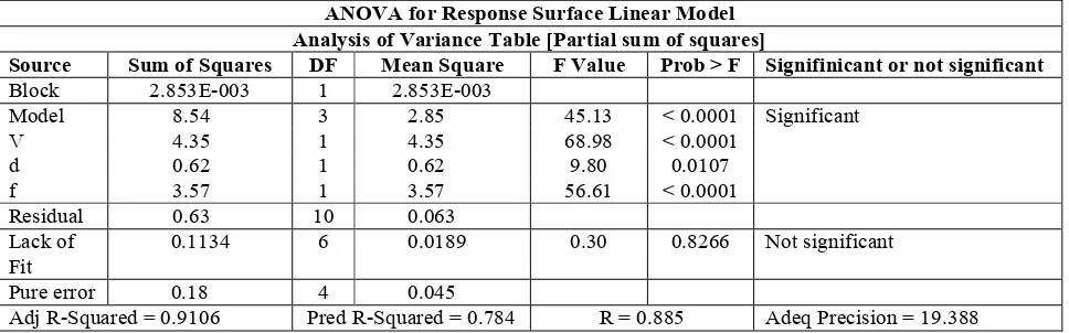
[image:7.595.52.536.271.422.2]

From Table 4 below, the Model F-value of 45.13 implies the model is significant. There is only a 0.01% chance that a "Model F-Value" this large could occur due to noise. Values of "Prob > F" less than 0.0500 indicate model terms are significant. In this case V, d, f are significant model terms. Values greater than 0.1000 indicate the model terms are not significant. If there are many insignificant model terms (not counting those required to support hierarchy), model reduction may improve your model. The "Pred R-Squared" of 0.7840 is in reasonable agreement with the "Adj R-Squared" of 0.9106. "Adeq Precision" measures the signal to noise ratio. A ratio greater than 4 is desirable. Your ratio of 19.388 indicates an adequate signal. The "Lack of Fit F-value" of 0.30 implies the Lack of Fit is not significant relative to the pure error. There is a 82.66% chance that a "Lack of Fit F-value" this large could occur due to noise. Non-significant lack of fit is good -- we want the model to fit.

Table 4: ANOVA of 1st _{order (linear) CCD Model}

ANOVA for Response Surface Linear Model Analysis of Variance Table [Partial sum of squares]

Source Sum of Squares DF Mean Square F Value Prob > F Signifinicant or not significant

Block 2.853E-003 1 2.853E-003

Model 8.54 3 2.85 45.13 < 0.0001 Significant

V 4.35 1 4.35 68.98 < 0.0001

d 0.62 1 0.62 9.80 0.0107

f 3.57 1 3.57 56.61 < 0.0001

Residual 0.63 10 0.063

Lack of Fit

0.1134 6 0.0189 0.30 0.8266 Not significant

Pure error 0.18 4 0.045

Adj R-Squared = 0.9106 Pred R-Squared = 0.784 R = 0.885 Adeq Precision = 19.388

4.2.2. Checking the adequacy of the quadratic model

[image:8.595.67.549.107.316.2]

Table 5: ANOVA of 2st _{order (Quadratic) CCD Model}

ANOVA for Response Surface Quadratic Model Analysis of Variance Table [Partial sum of squares] Source Sumof

Squares DF Mean Square F Value Prob > F

Signifinicant or not significant

Block 2.853E-003 1 2.853E-003

Model 9.14 7 1.31 299.22 < 0.0001 significant

V 2.80 1 2.80 642.01 < 0.0001

d 0.78 1 0.78 179.78 < 0.0001

f 3.57 1 3.57 817.88 < 0.0001

d2 _{0.062 1 0.062 14.11 0.0094}

f2 _{0.23 1 0.23 52.85 0.0003}

Vf 0.22 1 0.22 49.85 0.0004

df 0.079 1 0.079 18.19 0.0053

Residual 0.026 6 4.365E-003

Lack of Fit 1.833E-003 2 9.166E-004 0.21 0.6513 Not significant

Pure error 0.071

Adj -Squared = 0.9938 Pred R-quared = 0.8523 R = 0.923 Adeq Precision =

51.031

4.3. Checking the estimated of error of the developed model

[image:9.595.49.539.107.325.2]

Table 6: Experimental, Predicted and Error Values

Design cutting condition Response=Tool life (TL)(min) Error (ei) Trial

no. (T) Cutting speed (m/min)

Depth of

cut (mm) (mm/tooth)Feed Experim. values

Predicted value Linear Predicted value Quadratic Linear

model Quadratic model

1 72.28 1.63 0.025 27.83 20.69 26.05 0.26 0.06

2 72.28 0.61 0.079 8.81 9.76 9.03 -0.11 -0.03

3 44.27 1.63 0.079 25.16 24.49 25.47 0.03 -0.01

4 44.27 0.61 0.025 124.93 159.23 122.83 -0.27 0.02

5 56.57 1.00 0.044 30.30 30.08 31.88 0.01 -0.05

6 56.57 1.00 0.044 30.30 30.08 31.88 0.01 -0.05

7 56.57 1.00 0.044 30.30 30.08 31.88 0.01 -0.05

8 56.57 1.00 0.044 30.30 30.08 31.88 0.01 -0.05

9 56.57 1.00 0.044 30.30 30.08 31.88 0.01 -0.05

10 40.00 1.00 0.044 114.27 85.67 104.18 0.25 0.09

11 80.00 1.00 0.044 10.71 10.56 9.76 0.01 0.09

12 56.57 0.50 0.044 70.70 44.65 71.72 0.37 -0.01

13 56.57 2.00 0.044 20.20 20.26 20.37 0.00 -0.01

14 56.57 1.00 0.02 55.55 73.89 57.00 -0.33 -0.03

15 56.57 1.00 0.10 8.89 11.80 8.92 -0.33 0.00

Average of error (linear),





   ₁₅ 1 15 1 ) ( ) ( i i l el T trial of number Total e linear of error of Sum Avg (10) 15 33 . 0 ... 11 . 0 26 .

0   



el Avg

= 0.08

Standard deviation (linear),





    1 ) ( . ) ( 15 1 T trial of No error linear of average error linear of trial each Std i l (11)

= 0.183

Average of error (quadratic),





   ₁₅ 1 15 1 ) ( ) ( i i q eq T trial of number Total e quadratic of error of Sum Avg (12) 15 00 . 0 ... 06 . 0 06 .

0   



eq Avg

Standard deviation (quadratic), Stdq =





   

1 ) ( .

) (

15

1

T trial of No

error quadratic of

average quadratic

linear of trial each

Std i

q (13)

= 0.028

5. Conclusions

This research work was undertaken to develop a mathematical relationship between the tool life in end milling of hard material (AISI D2) and the machining variables by using the experimental results obtained through use of the concept of RSM. It has been possible to develop the first order (linear model) as well as the second order (quadratic model). Adequacy or validity of the models has been evaluated by ANOVA which indicates that the models are reliable. These models can be safely used to predict the tool life of the machined part of AISI D2 tool steel under the specified cutting conditions. These models are valid within the ranges of the cutting parameters in end milling which for cutting speed range is 40 - 80 m/min, for depth of cut range is 0.5 - 2.0 mm and for feed range is 0.05 - 0.1 mm/tooth. Both models linear (1st order) and CCD quadratic (2nd order) have shown similar trends indicating that the cutting speed has the most significant influence on tool life followed by feed and depth of cut. Hence, the percentage average of error between the predicted and measured tool life of both models is less than 10% but for quadratic model we found the average percentage error is less than 5%. Finally, a reliable technique for modelling tool life knowledge in end milling operations has been demonstrated in this paper.

Acknowledgement

References

[1] Becze, C.E.; Clayton, P.; Chen, L.; El-Wardany, T.I.; Elbestawi, M.A. (2000). High-speed five-axis milling of hardened tool steel, International Journal of Machine Tools & Manufacture, 40: 869-885.

[2] Benardos, P.G. & Vosniakos, G.C. (2003). Predicting surface roughness in machining: a review,

International Journal of Machine Tools & Manufacture, 43: 833-844.

[3] Bhatia, S.M.; Pandey, P.C.; Shan, H.S. (1979). Failure of cemented carbide tools in intermittent cutting, Journal of Precision Engineering, 148-152.

[4] Ee, K.C.; Li, P.X.; Balaji, A.K.; Jawahir, I.S.; Stevenson, R. (2006). Performance-based predictive models and optimization methods for turning operations and application: Part 1 – Tool wear/tool life in turning with grooved tools, Journal of Manufacturing Processes, SME, Vol.8/No.1: 54-66. [5] Eldem, S.; Barrow, G. (1976). Tool life in interrupted turning operations, Israel Journal

Technology, 14:172-178

[6] Ghani, J.A.; Choudhury, I.A.; Masjuki, H.H. (2004). Performance of P10 TiN coated carbide tools when end milling AISI H13 tool steel at high cutting speed, Journal of Material Processing Technology, 153-154: 1062-1066.

[7] Ghani, J.A.; Choudhury, I.A.; Masjuki, H.H. (2004a). Wear mechanism of TiN coated carbide and uncoated cermets tools at high cutting speed application, Journal of Material Processing Technology, 161-162: 30-37.

[8] ISO Standard 8688-2 (1989). International Standard For Tool Life Testing In End Milling, Part-2, First edition 1989-05-01.

[9] Jawahir, I.S.; Wang, X. (2007). Development of hybrid predictive models and optimization techniques for machining operations, Journal of Material Processing Technology, 185:46-59. [10] Li, H.Z.; Zeng, H.; Chen, X.Q. (2006). An experimental study of tool wear and cutting force

variation in the end milling of inconel 718 with coated carbide inserts, Journal of Material Processing Technology, 180:296-304.

[11] Lopez de Lacalle, L.N.; Lamikiz, A.; Sanchez, J.A.; Arana, J.L. (2002). Improving the surface finish in high-speed milling of stamping dies, Journal of Material Processing Technology, 123: 292-302.

[12] Palanisamy, P.; Rajendran, I.; Shanmugasundaram, S. (2007). Prediction of tool wear using regression and ANN models in end-milling operation, International Journal of Advanced Manufacturing Technology, Springer-Verlag London, 10.1007.

[13] Ping, Y.C.; Yeong D.H. (1997). An improvement neural network model for the prediction of cutting tool life, Journal of Intelligent Manufacturing, 8: 107-115.

[14] Raymond, H. Myers & Douglas, C. Montgomery (2002). Response surface methodology: Process and product optimization using designed experiments, 2nd _{edition, John Wiley & Sons, USA.}

[15] Shaw, M.C. (2005). Metal cutting principles, Oxford publisher, New York.

[16] Tsai, M.K.; Lee, B.Y.; Yu, S.F. (2005). A predicted modelling of tool life of high-speed milling for SKD61 tool steel, International Journal of Advanced Manufacturing Technology, Springer-Verlag London, 26:711-717

[17] Vivancos, J.; Luis, C.J.; Ortiz, J.A.; Gonzalez, H.A. (2005). Analysis of factors affecting the high-speed side milling of hardened die steels, Journal of Material Processing Technology, 162-163: 696-701.

[18] Mansour, A. & Abdalla, H. (2002). Surface roughness for end milling: a semi-free cutting carbon casehardening steel (EN32) in dry condition, Journal of Material Processing Technology, 124: 183-191.