A new smoothing modified three term conjugate gradient method for \(l {1}\) norm minimization problem

R E S E A R C H

Open Access

A new smoothing modified three-term

conjugate gradient method for

l

₁

-norm

minimization problem

Shouqiang Du

_{and Miao Chen}

*_{Correspondence:}

[email protected] 1_{School of Mathematics and}

Stochastic, Qingdao University, Qingdao, China

Abstract

We consider a kind of nonsmooth optimization problems withl1-norm minimization, which has many applications in compressed sensing, signal reconstruction, and the related engineering problems. Using smoothing approximate techniques, this kind of nonsmooth optimization problem can be transformed into a general unconstrained optimization problem, which can be solved by the proposed smoothing modified three-term conjugate gradient method. The smoothing modified three-term conjugate gradient method is based on Polak–Ribière–Polyak conjugate gradient method. For the Polak–Ribière–Polyak conjugate gradient method has good numerical properties, the proposed method possesses the sufficient descent property without any line searches, and it is also proved to be globally convergent. Finally, the numerical experiments show the efficiency of the proposed method.

MSC: 90C30; 90C33

Keywords: Nonsmooth optimization problem; Smoothing modified three-term conjugate gradient method; Global convergence

1 Introduction

In this paper, we consider the following nonsmooth optimization problems withl1-norm

minimization problem

min x∈Rn

1

2Ax–b

2

2+τx1, (1)

wherex∈Rn_,A∈Rm×n_(mn),b∈Rm_{,τ> 0,v2denotes the Euclidean norm ofvand} v1=n_i=1|vi|is thel1-norm ofv. This problem is widely used in compressed sensing,

signal reconstruction, analog-to-information conversion and related to many mathemati-cal problems [1–16]. Problem (1) is also a typimathemati-cal compressed sensing scenario, which can reconstruct a length-nsparse signal frommobservations. From the Bayesian perspective, problem (1) can also be seen as a maximum a posteriori criterion for estimatingxfrom ob-servationsb=Ax+ω, whereωis the Gaussian noise of varianceσ2. Many researchers have studied the numerical algorithms, which can be used to solve problem (1) with large-scale data such as fixed point method [1], gradient projection method for sparse reconstruction [2], interior-point continuation method [3, 4], iterative shrinkage thresholds algorithms in

[5, 6], linearized Bregman method [7, 8], alternating direction algorithms [9], nonsmooth equations-based method [10] and some related methods [11, 12]. Just recently, a smooth-ing gradient method has been given for solvsmooth-ing problem (1) based on the new transformed absolute value equations in [14, 15]. The transformation is based on the equivalence be-tween a linear complementarity problem and an absolute value equation problem [17, 18]. The complementarity problem, the absolute value equation problem, and the related constrained optimization problem are three kinds of important optimization problems [19–23]. On the other hand, the nonlinear conjugate gradient methods and smoothing methods are used widely to solve large-scale optimization problems [24, 25], total varia-tion image restoravaria-tion [26], monotone nonlinear equavaria-tions with convex constraints [27], and nonsmooth optimization problems, such as nonsmooth nonconvex problems [28], minimax problem [29], P0 nonlinear complementarity problems [30]. Specially, the effec-tiveness of widely used and attained different numerical outcomes three-term conjugate gradient method, which is based on Hang–Zhang conjugate gradient method and Polak– Ribière–Polyak conjugate gradient method [31–33], has been widely studied. Based on the above analysis, in this paper, we propose a new smoothing modified three-term conjugate gradient method to solve problem (1). The global convergence analysis of the proposed method is also presented.

The remainder of this paper is organized as follows. In Sect. 2, we give the transfor-mation of problem (1), which includes the transfortransfor-mation of a linear complementarity problem transformed into an absolute value equation problem. In Sect. 3, we present the smoothing modified three-term conjugate gradient method and give the convergence analysis of it. Finally, we give some numerical results of the given method which show the effectiveness of it.

2 Results: the transformation of the problem

In this section, as in [9, 10, 14, 15], we set

x=u–v, u≥0,v≥0,

whereui= (xi)+ andvi= (–xi)+ for alli= 1, 2, . . . ,nwith (xi)+=max{xi, 0}. And we also

havex1= 1T

nu+ 1Tnv, where 1n= [1, 1, . . . , 1]Tis ann-dimensional vector with n ones.

Thus, problem (1) can be transformed into the following problem:

min z=(u,v)T_≥0

1

2b–Az

2

2+τ1Tnu+τ1Tnv,

i.e.,

min z≥0

1 2z

T_Hz+cT_{z, (2)}

where

z= (u,v)T, c=τ12n+

–c–

c–

, c=ATb, H=

AT_{A –A}T_A

–AT_{A A}T_A

SinceHis a positive semi-definite matrix, problem (2) can be translated into a linear vari-able inequality problem, which is to findz∈R2n_{such that}

Hz+c,˜z–z ≥0, ∀˜z≥0. (3)

By the feasible structure of the feasible region ofz, problem (3) is equivalent to the linear complementary problem, which to findz∈R2nsuch that

z≥0, Hz+c≥0, zT(Hz+c) = 0. (4)

Due to the equivalence of linear complementarity problems and absolute value equation problems, problem (4) can be transformed into the following absolute value equation problem, which is defined by

(H+I)z+c=(H–I)z+c.

Then problem (1) can be transformed into the following problem:

min z∈R2nf(z) =

1

2(H+I)z+c–(H–I)z+c

2

. (5)

3 Main results and discussions

In this section, we present the smoothing modified three-term conjugate gradient method to solve problem (1). Firstly, we give the definition of smoothing function and smoothing approximation function of the absolute value function [14, 15, 29].

Definition 1 Letf :Rn_{→Rbe a local Lipschitz continuous function. We call} ˜_{f :R}n_×

R+→Ra smoothing function off, if lim

μ→0f˜(x) =f(x),

wherefμ(·) is continuously differentiable inRnfor any fixedμ> 0.

The smoothing function of the absolute value function is defined by

iμ(z) =

(H–I)z+c 2_i+μ2_{, μ∈R}

+,i= 1, 2, . . . , 2n, (6)

and satisfies

lim

μ→0iμ(z) =(H–I)z+c i, i= 1, 2, . . . , 2n.

Based on (6), we obtain the following unconstrained optimization problem:

min z∈R2n ¯

fμ(z) =

1 2

2n

i=1 ¯

f_iμ2(z),

wheref¯iμ(z) = ((H+I)z+c)i–iμ(z) is a smoothing function off(z) in (5) fori= 1, 2, . . . , 2n.

Algorithm 1(Smoothing modified three-term conjugate gradient method)

Step 0. Choose0 <σ< 1,0 <ρ< 1,r> 0,μ= 2,η= 1,ε> 0,μ0> 1and, given an initial

pointz0∈Rn, letd0= –g˜0, whereg˜0=∇zf˜(z0,μ0).

Step 1. If∇zf˜ ≤ε, stop; otherwise, go to Step 2.

Step 2. Compute search direction by usingβ˜_kBZAUandθ˜_kBZAU, which are defined by

˜

β_kBZAU= ∇Zf˜μ(zk)

T_(∇Zf˜

μ(zk) –∇Zf˜μ(zk–1))

–η∇Zf˜μ(zk–1)Tdk–1+μ|∇Zf˜μ(zk)Tdk–1|

, (7)

˜

θ_kBZAU= ∇Zf˜μ(zk)

T_d k–1

–η∇Zf˜μ(zk–1)Tdk–1+μ|∇Zf˜μ(zk)Tdk–1|

, (8)

dk=

–∇Zf˜μ(zk) ifk= 0,

–∇Zf˜μ(zk) +β˜kBZAUdk–1–θ˜kBZAUyk–1 ifk≥1,

whereyk–1=∇Zf˜μ(zk) –∇Zf˜μ(zk–1).

Step 3. Computeαkby the Armijo line search, whereαk=max{ρ0,ρ1,ρ2, . . .}andρi

satisfies

˜

fzk+ρidk,μk ≤ ˜f(zk,μk) +σρi∇Zf˜μ(zk)Tdk. (9)

Step 4. Computezk+1=zk+αkdk, if∇zf¯(zk+1,μk) ≥rμk, setμk+1=μk. Otherwise, let

μk+1=σ μk.

Step 5. Setk:=k+ 1and go to Step 1.

Now, we give convergence analysis of Algorithm 1. In order to get the global convergence of Algorithm 1, we give the following assumptions.

Assumption 1

(i) The level set={z∈R2n|˜fμ(z)≤ ˜fμ(z0)}is bounded.

(ii) There exists a positive constantL> 0such that∇Zf˜μ(zk)is Lipschitz continuous on

an open convex setB⊆and for anyz1,z2∈B, i.e.,

_∇Zf˜μ(z1) –∇Zf˜μ(z2)≤Lz1–z2.

(iii) There exists a positive constantmsuch that

mdx2≤dT∇_z2f˜μ(zk)dk, ∀x,d∈Rn,

where∇2

zf˜μ(zk)is the Hessian matrix off˜.

By Assumption 1, we can see that there exist positive constantsγ > 0 andbsuch that

_∇Zf˜μ(zk)≤γ, ∀zk∈

and

Lemma 1 Suppose{zk}and{dk}are generated by Algorithm1,then

∇Zf˜μ(zk)Tdk= –∇Zf˜μ(zk) 2

and

_∇Zf˜μ(zk)≤ dk.

Proof By Algorithm 1, we have

dk= –∇Zf˜μ(zk) +β˜kBZAUdk–1–θ˜kBZAUyk–1.

Multiplying both sides of the above equation by∇Zf˜μ(zk)T, we obtain

∇Zf˜μ(zk)Tdk= –∇Zf˜μ(zk) 2

+∇Zf˜μ(zk)

T_(∇Zf˜

μ(zk) –∇Zf˜μ(zk–1))(∇Z˜fμ(zk)Tdk–1)

–η∇Zf˜μ(zk–1)Tdk–1+μ|∇Zf˜μ(zk)Tdk–1|

–(∇Zf˜μ(zk)

T_d

k–1∇Zf˜μ(zk)T(∇Zf˜μ(zk) –∇Zf˜μ(zk–1))

–η∇Zf˜μ(zk–1)Tdk–1+μ|∇Z˜fμ(zk)Tdk–1|

,

i.e.,

∇Zf˜μ(zk)Tdk= –∇Zf˜μ(zk) 2

.

Now, we have

_∇Zf˜μ(zk)Tdk=∇Zf˜μ(zk) 2

and

_∇Zf˜μ(zk)Tdk≤∇Zf˜μ(zk)dk.

By

_∇Zf˜μ(zk) 2

≤∇Zf˜μ(zk)dk

we have

_∇Zf˜μ(zk)≤ dk.

Hence, the proof is complete.

Lemma 2 Suppose Assumption1holds and{zk}and{dk}are generated by Algorithm1,

then

∞

k=0

and

∞

k=0

∇Zf˜μ(zk)4 dk2 < +∞.

Proof Using the techniques similar to lemmas in [31–33], we can get this lemma. The

description will not be repeated again.

Lemma 3 Suppose Assumption1holds and xkand dkare generated by Algorithm1,then

a1αkdk2≤–∇Zf˜μ(zk)Tdk, (10)

where a1= (1 –σ)–1(m/2),m is a positive constant and0 <σ< 1.

Proof By using Taylor’s expansion, we have

˜

f(zk+1) =f˜(zk) +∇Zf˜μ(zk)Tsk+

1 2s

T

kGksk, (11)

wheresk=zk+1–zk=αkdkand

Gk=

1

0 ∇2

zf˜μ(zk+τsk)dτsk.

By Armijo line search, we know that

˜

f(zk+1)≤ ˜f(zk) +σ∇zf˜μ(zk)Tsk. (12)

By (11) and (12), we have

1 2s

T

kGksk≤(1 –σ)

–∇Zf˜μ(zk)Tsk ,

i.e.,

1 2(1 –σ)

–1_mαkdk2_≤–∇Zf˜

μ(zk)Tdk.

Denotea1= (1 –σ)–1(m/2), we get (10). Thus, we complete the proof.

By Lemmas 1, 2, and 3, we can get global convergence of the given method, i.e., the following theorem.

Theorem 1 Suppose Assumption1holds,then

lim k→∞

_∇Zf˜μ(zk)= 0.

Proof From Assumption 1, (7), and (10), we have

β˜_kBZAU≤∇Zf˜μ(zk) T_(∇Zf˜

μ(zk) –∇Zf˜μ(zk–1))

η(–∇Zf˜μ(zk–1)Tdk–1)

≤∇Zf˜μ(zk)Lαk–1dk–1

η(a1αk–1dk–12)

β˜_kBZAUdk–1 ≤

L∇Zf˜μ(zk)

η(a1dk–1)

dk–1=L∇Zf˜μ(zk) ηa1

,

i.e.,

θ˜_kBZAUyk–1 ≤ ∇Zf˜μ(zk)

T_d k–1

η(–∇Zf˜μ(zk–1)Tdk–1)

yk–1.

From Assumption 1, (8), and (10), we have

θ˜_kBZAUyk–1 ≤

_∇Z˜

fμ(zk)Lxk–xk–1

η(a1αk–1dk–12)

dk–1=L∇Zf˜μ(zk) ηa1

. (14)

Combining (13), (14), anddkgenerated in Algorithm 1, we obtain dk ≤∇Z˜fμ(zk)+β˜kBZAUdk–1+θ˜kBZAUyk–1

≤∇Z˜fμ(zk)+

L∇Zf˜μ(zk)

ηa1

+L∇Zf˜μ(zk) ηa1

=

1 + 2L ηa1

∇Zf˜μ(zk).

Denote√B= (1 +_ηa2L

1), we havedk

2_≤B∇Zf˜

μ(zk)2, i.e.,

1

dk2≥

1

B∇Zf˜μ(zk)2

and

B∇Zf˜μ(zk)4 dk2 ≥

∇Z˜fμ(zk)4

˜gk2 =∇Zf˜μ(zk) 2

By Lemma 2, we have

∞

k=0

_∇Zf˜μ(zk) 2

< +∞.

This completes the proof.

4 Numerical experiments

Example1 Consider

A=

⎛ ⎜ ⎜ ⎜ ⎝

3 5 8 4 1 5 2 9 6 5 7 4 3 4 7 2 1 6 8 9 6 5 7 4

⎞ ⎟ ⎟ ⎟

⎠, b= ( 2 4 1 7 )T,

andτ= 5.

From [14], we know that this example has a solutionx∗= (0.3461, 0.0850, 0, 0, 0.3719, 0)T_.

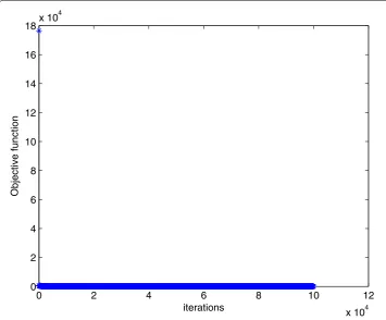
The optimal solution of Algorithm 1 is x∗ = (0.3459, 0.0850, 0.0001, 0.0009, 0.3717, –0.0001)T_{. In Figs. 1 and 2, we plot the evolution of the objective function versus the}

number of iterations when solving Example 1 with Algorithm 1 and the smoothing gradi-ent method respectively.

Example2 Consider

A=

⎛ ⎜ ⎜ ⎜ ⎜ ⎝

1 1 1 0 0 0 · · · 0 0 0 1 · · · 1 0 0 0 1 1 1 · · · 0 0 0 1 · · · 1

..

. ... ... ... ... ... · · · ... ... ... ... · · · ... 0 0 0 0 0 0 · · · 1 1 1 1 · · · 1

⎞ ⎟ ⎟ ⎟ ⎟ ⎠

m×n

,

b= ( 1 1 · · · 1 )T,

Figure 2Numerical results for solving Example 1 with smoothing gradient method

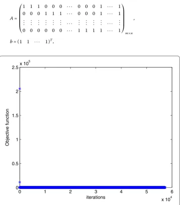
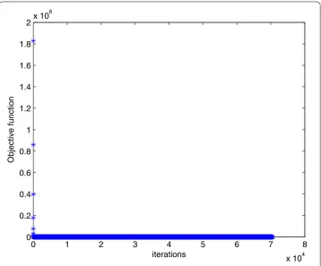
andτ= 2. In this example, we choosem= 30,n= 100. The numerical results are given in Figs. 3 and 4.

Example3 Consider

A= ⎛ ⎜ ⎜ ⎜ ⎜ ⎜ ⎜ ⎜ ⎝

1 0 · · · 0 1 1 · · · 1 0 1 · · · 1 0 1 · · · 1

..

. ... . .. ... ... ... · · · ... 0 1 · · · 1 0 1 · · · 1 1 0 · · · 0 1 1 · · · 1

⎞ ⎟ ⎟ ⎟ ⎟ ⎟ ⎟ ⎟ ⎠

m×n

, b= ( 1 1 · · · 1 )T,

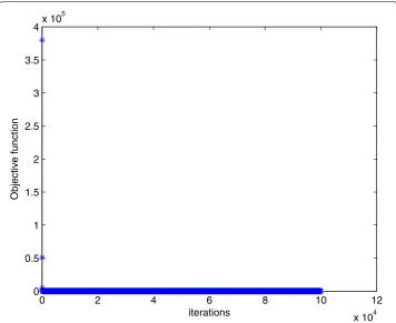
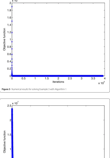
andτ = 6. In this example, we choosem= 100,n= 110. The numerical results are given in Figs. 5 and 6.

Example4 Consider

A= ⎛ ⎜ ⎜ ⎜ ⎜ ⎜ ⎜ ⎜ ⎜ ⎝

4 –1 0 · · · 0 1 · · · 1

–1 4 –1 · · · ... ... · · · ...

0 –1 4 . .. ... ... · · · ... ..

. . .. ... ... –1 ... · · · ... 0 · · · 0 –1 4 1 · · · 1

⎞ ⎟ ⎟ ⎟ ⎟ ⎟ ⎟ ⎟ ⎟ ⎠

m×n

Figure 3Numerical results for solving Example 2 with Algorithm 1

Figure 5Numerical results for solving Example 3 with Algorithm 1

Figure 7Numerical results for solving Example 4 with Algorithm 1

Figure 9Numerical results for solving Example 5 with Algorithm 1

andτ= 10. In this example, we choosem= 200,n= 210. The numerical results are given in Figs. 7 and 8.

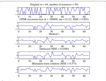
Example5 In this example, we consider a typical compressed sensing problem, which is also considered in [9, 10, 14, 15]. In this example, we choosem= 24_{,n= 2}6_{,σ= 0.5,ρ= 0.4,}

γ = 0.5,ε= 10–6_{,μ= 5,η= 2. The original signal contains 520 randomly generated±1}

spikes. Further, them×nmatrixAis obtained by first filling it with independent samples of a standard Gaussian distribution and then orthogonalization of its rows. In this example, we choose σ2= 10–4 _{andτ = 0.1A}T_y

∞ the same as suggested in [14]. The numerical

results are shown in Fig. 9.

5 Conclusion

In this paper, we have proposed a new smoothing modified three-term conjugate gradient method for solvingl1-norm nonsmooth problems. Comparing with the smoothing

gradi-ent method, GPSR method, and other methods proposed in [2, 9, 10, 14], we can see that the smoothing modified three-term conjugate gradient method is simple and needs small storage. Comparing with the smoothing gradient method proposed in [14], the smoothing modified three-term conjugate gradient method is significantly faster especially in solving large-scale problems.

Acknowledgements

This work was supported by the National Natural Science Foundation of China (No. 11671220) and the Natural Science Foundation of Shandong Province (No. ZR2016AM29).

Competing interests

Authors’ contributions

All authors contributed equally. All authors read and approved the final manuscript.

Publisher’s Note

Springer Nature remains neutral with regard to jurisdictional claims in published maps and institutional affiliations.

Received: 26 February 2018 Accepted: 21 April 2018

References

1. Hale, E.T., Yin, W., Zhang, Y.: Fixed-point continuation forl1-minimization: methodology and convergence. SIAM J. Optim.19(3), 1107–1130 (2008)

2. Figueiredo, M.A.T., Nowak, R.D., Wright, S.J.: Gradient projection for sparse reconstruction, application to compressed sensing and other inverse problems. IEEE J. Sel. Top. Signal Process.1(4), 586–597 (2007)

3. Kim, S.J., Koh, K., Lustig, M., Boyd, S., Gorinevsky, D.: An interior-point method for large-scalel1-regularized least squares. IEEE J. Sel. Top. Signal Process.4, 606–617 (2007)

4. Turlach, B.A., Venables, W.N., Wright, S.J.: Simultaneous variable selection. Technometrics47(3), 349–363 (2005) 5. Daubechies, I., Defrise, M., Mol, C.D.: An iterative thresholding algorithm for linear inverse problems with a sparsity

constraint. Commun. Pure Appl. Math.57(11), 1413–1457 (2004)

6. Beck, A., Teboulle, M.: A fast iterative shrinkage-thresholding algorithm for linear inverse problems. SIAM J. Imaging Sci.2, 183–202 (2009)

7. Osher, S., Mao, Y., Dong, B., Yin, W.: Fast linearized Bregman iteration for compressive sensing and sparse denoising. Math. Comput.8(1), 93–111 (2011)

8. Yin, W., Osher, S., Goldfarb, D., Darbon, J.: Bregman iterative algorithm forl1minimization with applications to compressed sensing. SIAM J. Imaging Sci.1(1), 143–168 (2008)

9. Yang, J., Zhang, Y.: Alternating direction algorithms forl1-problems in compressive sensing. SIAM J. Sci. Comput.33, 250–278 (2011)

10. Xiao, Y.H., Wang, Q.Y., Hu, Q.J.: Non-smooth equations based method forl1-norm problems with applications to compressed sensing. Nonlinear Anal.74(11), 3570–3577 (2011)

11. Wakin, M.B., Laska, J.N., Duarte, M.F., Baron, D., Sarvotham, S., Takhar, D., Kelly, K.F., Baraniuk, R.G.: An architecture for compressive imaging. In: 2006 International Conference on Image Processing, pp. 1273–1276 (2006)

12. Lustig, M., Donoho, D., Pauly, J.M.: Sparse MRI: the application of compressed sensing for rapid MR imaging. Magn. Reson. Med.58(6), 1182–1195 (2010)

13. Farajzadeh, A.P., Plubtieng, S., Ungchittrakool, K.: On best proximity point theorems without ordering. Abstr. Appl. Anal.2014, Article ID 130439 (2014)

14. Chen, Y.Y., Gao, Y., Liu, Z.M., Du, S.Q.: The smoothing gradient method for a kind of special optimization problem. Oper. Res. Trans.21(2), 119–125 (2017)

15. Chen, M., Du, S.Q.: The smoothing FR conjugate gradient method for solving a kind of nonsmooth optimization problem withl1-norm. Math. Probl. Eng.2018, Article ID 5817931 (2018)

16. Wang, Y.J., Zhou, G.L., Caccetta, L., Liu, W.Q.: An alternative Lagrange-dual based algorithm for sparse signal reconstruction. IEEE Trans. Signal Process.59(4), 1895–1901 (2011)

17. Mangasarian, O.L.: Absolute value programming. Comput. Optim. Appl.36(1), 43–53 (2007)

18. Mangasarian, O.L.: A generalized Newton method for absolute value equations. Optim. Lett.3(1), 101–108 (2009) 19. Caccetta, L., Qu, B., Zhou, G.L.: A globally and quadratically convergent method for absolute value equations.

Comput. Optim. Appl.48(1), 45–58 (2011)

20. Mangasarian, O.L.: Absolute value equation solution via concave minimization. Optim. Lett.1(1), 3–8 (2007) 21. Chen, H.B., Wang, Y.J., Zhao, H.G.: Finite convergence of a projected proximal point algorithm for generalized

variational inequalities. Oper. Res. Lett.40(4), 303–305 (2012)

22. Chen, Y.Y., Gao, Y.: Two kinds of new Levenberg–Marquardt method for nonsmooth nonlinear complementarity problem. ScienceAsia40, 89–93 (2014)

23. Qu, B., Xiu, N.H.: A relaxed extragradient-like method for a class of constrained optimization problem. J. Ind. Manag. Optim.3(4), 645–654 (2007)

24. Fleteher, R., Reeves, C.M.: Function minimization by conjugate gradients. Comput. J.7(2), 149–154 (1964)

25. Dai, Y.H., Yuan, Y.: A nonlinear conjugate gradient method with a strong global convergence property. SIAM J. Optim.

10(1), 177–182 (1999)

26. Yu, G.H., Qi, L.Q., Dai, Y.H.: On nonmonotone chambolle gradient projection algorithms for total variation image restoration. J. Math. Imaging Vis.35(2), 143–154 (2009)

27. Yu, Z.S., Lin, J., Sun, J., Xiao, Y.H., Lin, L.Y., Li, Z.H.: Spectral gradient projection method for monotone nonlinear equations with convex constraints. Appl. Numer. Math.59(10), 2416–2423 (2009)

28. Chen, X.J.: Smoothing methods for nonsmooth, nonconvex minimization. Math. Program.134, 71–99 (2012) 29. Pang, D.Y., Du, S.Q., Ju, J.J.: The smoothing Fletcher–Reeves conjugate gradient method for solving finite minimax

problems. ScienceAsia42, 40–45 (2016)

30. Zhang, L., Wu, S.Y., Gao, T.: Improved smoothing Newton methods forP0nonlinear complementarity problems. Appl. Math. Comput.215(1), 324–332 (2009)

31. Zhang, L., Zhou, W.: On the global convergence of the Hang–Zhang conjugate gradient method with Armijo line search. Acta Math. Sci.28(5), 840–845 (2008)

32. Sun, M., Liu, J.: Three modified Polak–Ribière–Polyak conjugate gradient methods with sufficient descent property. J. Inequal. Appl.2015, Article ID 125 (2015)