2018 3rd International Conference on Computational Modeling, Simulation and Applied Mathematics (CMSAM 2018) ISBN: 978-1-60595-035-8
Stability Analysis of Power System Based on GA-SVM
Zong-yang LIU
1,2, Meng CHEN
2and Chong-tao LI
21
State Grid Sichuan Electrical Power Research Institute, Sichuan, China
2
School of Electrical Engineering, Xi'an Jiaotong University, Xi'an, China
Keywords: Stability analysis, Power system, GA, SVM.
Abstract. Aiming at the problems of long calculation time and stable stability of power system
stability analysis, a GA-SVM algorithm is proposed to analyze the stability of power system. Firstly, the mathematical model is used to describe the power system. The GA algorithm is used to optimize the nonlinear regression SVM parameters. The stability of the power system is simulated and the accuracy and speed under different load levels are verified. The simulation results show that the proposed algorithm has good efficiency, good reliability and high engineering practicability.
Introduction
Nowadays, as the scale of power networks is growing and the structure is becoming more complex, the issues of security and stability are becoming more prominent. At the same time, the rapid development of intelligent algorithms provides a broader choice for power system stability analysis
[1-3]
. In this paper, GA algorithm optimizes power system stability parameters, and uses support vector machine (SVM) to improve the accuracy and efficiency of power system stability analysis. A GA-SVM-based model can be used to evaluate the stability of power system in real time. The simulation results prove the effectiveness of the algorithm.
Power System Mathematical Description
The power system is characterized by nonlinearity, poor tolerance and lack of effective models. It is a typical nonlinear system, which can be described by the following high-dimensional nonlinear
differential algebraic equations with parameters[4]:
(x, y, z) 0 (x, y, z)
X f g
(1)
Where x is the state variable of the system, such as the motion variable, the rotor angle and the rotor angular velocity, and may also include the controlled internal electromotive force E'd, E'q, etc.; y is an algebraic variable, such as the current Id in the generator, Iq, voltage amplitude and phase angle of other busbars, etc., z is a parameter, which can be a device parameter, or an operating parameter, such as the active power or reactive power of the load. Differential equations describe the dynamic behavior of dynamic components, and algebraic equations reflect the interaction between dynamic components and network topology constraints. When considering the role of the digital controller and the discrete behavior of other components of the power system, it must also be described by a difference equation, so the power system becomes a hybrid system, which can be described by a nonlinear differential-differential-algebraic equation system.
GA Algorithm Optimization Parameters
0101000101
: : Solution
space
NO
Solution space
YE S
Coding space
0100101001 1001011010 1001100100
1001100100
1101000101 1101101001 0011010011 0111101000 1001100100
Cross
Fitness End
judgement
Code Initialization
Select Crossover
Mutation
Optimun Evaluation
[image:2.595.152.438.73.211.2]function
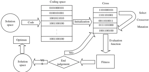
Figure 1. The calculation procedure of GA algorithm.
Coding
Binary coding is used. The discrete scope is set to be 3~8, 3 binary is used to express from 000 to 111. Suppose a total of 6 input-output variables x1,x2,x3,x4,y1,y2 , then the binary string:
011,010,001,101,100,000 respectively indicates that the partition number of x1 is bin2dec (011) +2 =
5, (bin2dec () is a function which binary string converted to a decimal number), similarly, the partition number of x2 is 4, the partition number of x3 is 3, the partition number of x4 is 7, the partition
number of y1 is 6, the partition number of y2 is 2, the discretization degree of input-output is recorded as [7 6 3 4 5 2].
Fitness function
Each chromosome (binary string) corresponds to a fuzzy neural network, the generalization results
) (s
J of the neural network is used to construct a fitness function which measures the fitness of
chromosome. Set the fitness function f
s 1/J
s , and s is a binary string, J
s indicates thebinary string corresponding to the generalization results of neural network. J
s is defined as follows:
Nt
i
i i t
y y N s
J
1
2 '
1 ) (
,
xi,yi
Stest (2)In the formula,Stest xiyi,i1,2,,Nt is the test sample sets; Nt is the test sample number; yi is
the actual value; yi' is the output of neural networks.
Evolutionary process
Firstly, generate randomly initial population. Calculate each individual's fitness of the initial population, then obtain breeding population through the competitive strategies of survival, that is, choose two individuals randomly from the initial population, individuals who have large fitness will
join the breeding population with probability of Ps, individuals who have small fitness will join the
breeding population with probability of 1Ps
0.6Ps1
.Termination criterion
Stability Analysis Based on Non-Regression SVM
The nonlinear data is mapped to the high-dimensional space by the kernel function, and the linear regression is performed in the high-dimensional space. Similarly, the quadratic programming optimization form as follows:
) ( ) ( ) )( , ( ) ( 2 1 ) , ( min 1 1 * * 1 , * * *
n i n i i i i i i n j i j j j i T ii K x x y
w
(3) the support vector regression estimation function is
n i i ii K x x b
x f 1 *) ( , ) ( ) ( (4) *
( ) (0, )
( ) (0, )
i i i
i i i
b y w x a C
b y w x a C
(5)
In the support vector regression estimation of real-valued functions, the number of support vectors is value-controlled. Suppose that the function is approximated by precision, that is, the function is described by an estimation function, so that the function is in the pipeline. To construct such a function, you can take an elastic pipe (the pipe always tends to be flat) and put the function into the pipe. The kernel function describes the elastic law of the pipe. The axis of this pipe defines the approximation of the function. Since the support vectors are those in which the Lagrangian multiplier is not zero in the KKT condition, and this multiplier defines the boundary point in the optimization problem of the inequality type, that is, the point at which the function touches the pipe, so The coordinates of the point at which the pipe encounters the function can be considered to define the support vector. The larger the value, the wider the pipe and the fewer contact points, ie the fewer support vectors.
If a training sample set is given, n
n n y x y x y x
T 1, 1, 2, 2,, , , where
n
i R
x , yiR,
n
i1,, , suppose
n i i
emp y w x b
n b w R 1 ) ( 1 ) ,
( , then the empirical risk minimization under
constraints Remp(w,b)is equivalent to:
n i n i i i F 1 1 * *) , ( s.t i n
b x w y y b x w i i i i i i i i , , 1 , 0 , ) ) (( ) ) (( * * (6) Construct a Lagrangian function for the above formula:
) , , , , , , ,
(w* * C* *
L =
n i n i i i i i i
i y w x b
1 1 * ) [ ( ) ] ( n i n i i i
i c w w
C y b x w 1 * * * ] )) ( ( 2 ) [(
n i i i i i 1 * * ) ( (7)Solve the above formula, and find the minimum pointw, b, *
i
and ,find the maximum point for
the Lagrangian multipliers , C*0, i* 0, i 0, 0
*
i
and i 0(i1,,n) . The solution of the
) (
) ( 2 1 ) , , (
1 1
*
*
n
i n i
i i C w w
w
(8)
s.t. i n
b x w y
y b x w
i i
i i
i
i i i
, , 1 0 ,
) ) ((
) ) ((
*
*
The first item on the right side of the formula is to improve the generalization ability of learning, the second item is to reduce the error, and the constant C makes a compromise between the two.
According to the definition of the insensitive loss function , when the difference
betweenf(xi)(wxi)b andyi is not greater than the error, that is zero, when it is greater than, the
error is: f(xi)yi , it can also be seen that the optimization problem obtained at this time also has
sparse characteristics.
Simulation
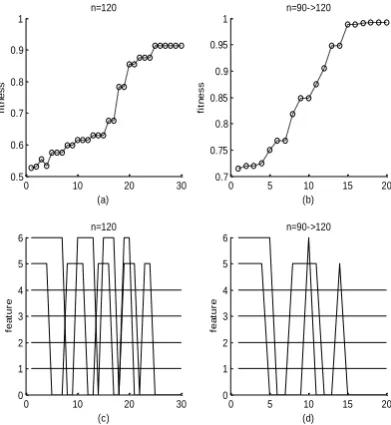
To test the effectiveness of the proposed algorithm, all experimental data was generated using the Power System Analysis Software Package (PSASP) for power system stability analysis. 90 and 120 samples were taken to form two sets of samples, and Figure 2 shows the actual training results. Figure 2 (a) and (c) are the fitness optimization changes when the sample data is 120; (b) and (d) are the number of fitness optimization changes from 90 samples to 120 samples. It can be seen in Fig. 2 that the optimal fitness of (a) and (b) is 0.9342 to 0.9948, respectively. It can be seen that the GA algorithm can reduce the optimal algebra and obtain better fitness value because the initial value of fitness is high. It helps the subsequent rapid optimization, and the GA algorithm prevents the irrelevant features from being repeatedly compared in the feature optimization process, and the fitness upward trend is stable, and the system optimization is very small.
0 10 20 30
0.5 0.6 0.7 0.8 0.9 1
n=120
(a)
fi
tn
e
ss
0 10 20 30
0 1 2 3 4 5 6
n=120
(c)
fe
a
tu
re
0 5 10 15 20
0.7 0.75 0.8 0.85 0.9 0.95 1
n=90->120
(b)
fi
tn
e
ss
0 5 10 15 20
0 1 2 3 4 5 6
n=90->120
(d)
fe
a
tu
[image:4.595.199.395.436.649.2]re
Figure 2. The change of fitness with the number of optimization times
Table 1. GA-SVM and BP neural network prediction results of power system stability.
Noise
Variance 0.2 0.4 0.4 0.8
GA-SV M
0.562 0.652 0.674 0.688
rm
s 0.0476 0.1121 0.1323 0.2331
BP Network
rms 0.0542 0.1229 0.1883 0.1090
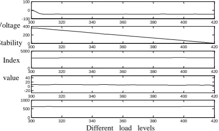
From the analysis results of power system stability of GA-SVM and BP neural network, it can be concluded that for Gaussian distributed noise, with the increase of noise variance, the accuracy of GAS-SVM power system stability analysis is significantly higher than that of BP neural network. It shows that GA-SVM has good anti-noise ability and function estimation and prediction performance. Fig. 3 shows the power system voltage stability index values for different load levels.
300 320 340 360 380 400 420
-100 0 100
300 320 340 360 380 400 420
0 200 400
300 320 340 360 380 400 420
0 5000
300 320 340 360 380 400 420
-20 0 20 40
300 320 340 360 380 400 420
0 500 1000
Figure 3. Power system voltage stability index values under different load levels.
Summary
In this paper, a GA-SVM method is proposed to study the stability of power system. In this method, GA algorithm is used to adaptively set the parameters of nonlinear regression SVM to improve the accuracy of SVM and improve the validity of calculation results. Compared with BP neural network, the calculation accuracy and efficiency of GA-SVM are better than BP neural network. The voltage stability index of power system under different load levels is also verified, which indicates that the proposed algorithm has a great application prospect.
References
[1] Acharya NV Rao PSN. A new voltage stability index based on the tangent vector of the power flowjacobian. 2013 IEEE Innovative Smart Grid Technologies-Asia (ISGT Asia). 2013.1-6.
[2] Patidar NP, Sharma J. Load ability margin estimation of power system using Model Trees. 2006 IEEE Power India Conference. 2006. 194:541-549.
[3] Han X, Zheng Z, Tian N, et a1. Voltage stability assessment based on BP neural network. Asia-Pacific Power & Energy Engineering Conference. 2009.1-4.
[4] Li Q. The Analysis and assessment of voltage stability based on GA-SVM. Journal of System Simulation, 2014, 10: 2369-2373.
[5] Sun J, Fang Palade K et a1. Quantum-behaved particle, swarm optimization with Gaussian distributed local attractor point. Applied Mathematics and Computation, 2011, 218(7): 3763-3775.
Voltage
Stability
Index
value
[image:5.595.176.398.258.391.2]