A Structure Sensitive Algorithm for Building Feature Line Extraction from LiDAR Data

2018 International Conference on Computer, Communication and Network Technology (CCNT 2018) ISBN: 978-1-60595-561-2

A Structure Sensitive Algorithm for Building Feature Line

Extraction from LiDAR Data

Chao HUANG

, Jing LI

, Wei ZHANG

, Min GUI

,

Pei-jun HUANG

and Jian-shun WANG

1

Xiamen Yilijiao Information Technology Co., Ltd, Xiamen, China

2

Wuhan University, Wuhan, China

*

Corresponding author

Keywords: Airborne LiDAR, Line detection, Structure sensitive algorithm, Building feature, Edge optimization, Hough transformation.

Abstract. Lines are important features for Airborne Laser Scanning (ALS) point clouds processing and model reconstruction, in which the lines are often detected by a Hough Transformation (HT) similar to in image processing. In fact, feature lines represent the edges of buildings, which are man-made objects and often have orthogonal, parallel and other relationships of regularity. In this paper, we propose a method for detecting and refining the line features from ALS data in consideration of these relationships of regularity. First, an angle and ρ voting algorithm is applied to conduct line detection to obtain the primary results. Second, an optimization process called structure sensitive competition, which relies on a line stability descriptor (LSD), refines the detected line segments. Finally, this proposed method is tested and compared to HT algorithm on a group of buildings with different complexity. The quality indicators, completeness, correctness and quality, show that the quality of the extracted lines can be substantially improved after the structure sensitive optimization.

Introduction

Three-dimensional building models are the primary data for city applications, e.g., digital city, security and protection, urban planning and visual navigation. Automatic reconstruction of detailed city models from remote sensing data is a hot research topic in the areas of photogrammetry and computer vision areas. Recently, airborne laser scanning (ALS, one type of LiDAR) technology, which is able to provide cloud data of directly measured Three-dimensional points, has been widely used in many areas, such as forest investigation, civil engineering and even cultural heritage. A LiDAR system shows great potential in building model reconstruction applications because it can acquire the points of a roof directly with reliable quality.

In this paper, the regularity and related stability of the line are employed as additional constrain information in the line feature detection. More specifically, we propose a structure sensitive line segment competition algorithm to optimize the results of the line detection in consideration of the regularity constraint and the line segments stability. At the beginning, the line features are extracted as the primary results for later post-processing by a line direction algorithm and a voting-based algorithm. Then, the line stability descriptor (LSD) is proposed; it can evaluate the stability of the detected lines by combining four elements, which are the length of the line, geometric regularity, number of points and fitting residual. Finally, a structure sensitive optimization is applied to all of the detected line segments. The processing in the final step can appear to be a competition of points between line segments. All of the points that belong to the detected line segments’ points will be re-evaluated, and some of the points will be re-assigned to the winner line segments based on the LSD.

Related Works

Originally, line detection was a primary step in the image processing and pattern recognition area. In 1962, Hough patented an algorithm for feature detection, which was later called the Hough Transformation (HT) [12], HT became one of the most famous and widely used algorithms of line feature detection. Since then, many papers and research studies have appeared about line feature detection in image using HT and optimized HT [13]. HT can appear to be a type of global search algorithm that detects lines by voting with each pixel for the possible lines in the line parameter space. This approach is effective, but it has heavy computational cost because all parameters must be exhaustively computed and stored in the algorithm. Later, Burns et al. [14] proposed a local search line extraction algorithm by connecting the line-support regions that consist of pixels with similar gradient orientations, which greatly speeds up the line extraction processing.

In terms of line feature detection from point clouds of a building, the line feature detection algorithms often have, at least partly, the goal of model reconstruction [6,7]. However, it is difficult to correctly extract the line features from airborne LiDAR data because the laser beam can seldom exactly hit the step edges of a building. In fact, the building edge points that are detected from airborne LiDAR data have much more noise than those from an optical image. The step edge that is located at the boundary of the building or the rooftops of multiple story buildings, where there are obvious height changes. They can be relatively easily detected from point clouds by testing the height changes. However, the step edge line feature detection often suffers from the noise points, e.g., plants, fences, air-conditions and other objects on the roofs.

For the purpose of building model reconstruction, some algorithms treat the step edges of a building as the boundary of the roof patches. [15] extract outline by projecting the points with a combination of a 2d cell grid and an angle criterion[16]. They trace the boundaries of the planar roofs and regularize the boundaries to create the building topological model [9,17]. However, these methods are vulnerable to the shape errors that are caused by the ubiquitous plants and furniture on the roofs which are very difficult to eliminate automatically.

To improve the quality of the line detection, the orthogonal relationships of the building line features are often employed to adjust the line detection results and enhance the results of the building model reconstruction. Vosselman [17] detected the boundary lines from airborne LiDAR data and use orthogonal rule to constrain the directions of the lines. The results show that the orthogonal constraint can greatly reduce the uncertainty of the detected lines. The orthogonal constraint is also used in [5] and [7] for line feature detection from imagery, although the projection of the image cannot strictly satisfy orthogonality.

This paper studies further the line extraction part of our previous work on building model reconstruction by considering the line stability and regularity in the extraction procedure [18]. In this paper, we assume that: 1) the points used in the line extraction belong to real world objects, which should follow many geometric constraints, for example, extracted line segments could not intersect each other; 2) regularity information between line segments should be utilized to augment the results of the line detection; and 3) residuals of fitted lines are very important to evaluate the stability of the extracted lines. Based on these assumptions, we define a stability descriptor for the detected lines and propose a competition algorithm to augment the quality of the extracted line features.

Methods

Figure 1 shows the flow chart of the algorithm that we proposed. First, the edge points, which were detected from the results of plane clustering by means of testing the Z values of border points [18], are given as the input to the voting procedure to extract the primary line segments. Then, the stability parameters of each line segments are calculated. Before the stability parameters computations, the relationships of the points to the line segments are constructed by the distance and connectivity in 2D space. The line segment computes only the points that are nearby or directly connected to it. The connectivity of the points to line segments can be obtained by the relationship of the point to point, which is built up by the Delaunay triangle network [19].. Based on the point-to-point relationships, point-to-line segment relationships can also be achieved. After this step, the stabilities of the lines are computed and the competition procedure is conducted. During the competition step, the labels of many points will be reassigned, accompanied by the post-processing steps, including the re-computation of the line parameters, and the line segments merging and breaking. The competition procedure stops when there is no point that needs to be assigned a new label. During this processing, if a line segment continuously loses points and reaches the limitation of the point number, e.g., 3 points, then that line will vanish, and all of the points in the line segment will degrade to isolated points.

Start

Point Voting to Detect Lines

Compute relation Between Points and Lines

Compute stability of each line

segments

Re-assign points to line Segments by points competition

Point Clouds

Line Segment Merging

Line Segment Breaks

Are Points Re-assigned?

End Yes

No

Voting based Line Extraction

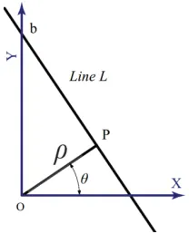
Basic Principles. In this section, we will introduce some basic geometric theory for later use. In the Cartesian coordinate system, a line can be represented by formula . In the polar coordinate system, the line is defined as equation 1.

(1) As shown in Figure 2, is the distance from the original point O to the line L. P is a projection of O onto the line. is the intersection angle of PO and the X axis. If the ρ can be given a negative value, then . In polar coordinates, the relation of , and b satisfy the equation below:

(2) In the polar coordinate representation, the two parameters and have finite space and thus it is easier for the points to vote the possible lines. In the algorithm implementation, a small problem must address the condition when is approaching zero, which means that the value of will be very sensitive to the existence of noise. However, this problem can be solved by mathematical skills.

Figure 2. Line parameters in the polar coordinate system.

Step Edge Point Detection and Point Parameters Estimation. The step edge points of buildings are detected by testing the Z values of the center point and its neighboring points. We employ the method in our previous paper to determine the step edge points [18]. This method detects the step edges points effectively, but it also brings many of the noise points to the resulting edge points. After the detection of the edge points, each point’s direction and ρ value is estimated by fitting the point sets that consist of the center point and its neighboring points. We assume that each point is a short “line segment”. Each of the short “line segments” casts a vote to support a possible line with certain parameters. If some of the lines obtain more votes than the given threshold, then this line will be deemed as a line feature candidate. The basic idea of this method is partly similar to the point voting based planar roof detection algorithm in [20], but the goal of voting here for line detection and the specific details is different.

As Figure 3 shows, for each edge point , we can search its adjacent points using Delaunay triangle mesh [19]. Additionally, a given distance threshold, e.g. twice the average point gap, is also used to limit the adjacent points into a local region. The average point gap computed

between two adjacent scan lines, and is the average distance between two adjacent points in a scan line. Similar to the angular criterion [16], the two consecutive adjacent points with maximum including angle and the center point are taken as a point set to estimate the point parameters. A least square line fitting algorithm is applied to this point set to compute the parameters of the short line in Cartesian space, as shown in Figure 3a, then the parameters are converted to polar space as parameters and as explained in section 3.1.1. The parameters θ and ρ of the line are given to point as well the fitting residual .

(3) To reduce the influence off the errors and noise, each point should be assigned with different weights in the line voting process according to its fitting residual. In view of this arrangement, a weight is assigned to the point by the fitting residual . Equation 3 is designed to give an appropriate weight to the point. In equation 3, the weight decreases while the increases, as shown in Figure 3b. The point with the residual beyond 2σ (σ is point placement accuracy) is considered as outlier that should be excluded.

(a) (b)

Figure 3. Weight of the point is decided by the distance to the fitted line. (a) shows the distance of the point to the line segment, and (b) is the segmented weight function.

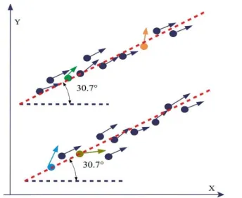
Figure 4. Each point cast a vote for possible line direction.

Here, the detailed techniques are explained. The θ and ρ value are estimated separately in two steps is similar to the method of plane detection [3]. First, we look for possible θ peaks only and determine which points that have equal θ values. Each peak represents a group of points that have the same direction, but could have different ρ values. Then, a new θ value is estimated by computing the average weighted θ values. Second, based on the new θ, new ρ value for each point is re-calculated. In this process, all of the involved points will be assigned the same θ but a new ρ. Finally, we determine peaks of group points by the histogram statistics of the ρ value of all of the points and we fit them into lines. This two-step procedure is slightly complex, but it generates more stable results. The reason is that θ and ρ are two correlated parameters with the covariant x, y, as formula 4 shows. If θ has error , the change of ρ value will be magnified by an error propagation:

Figure 5. “Angle repairing” processing helps determine the correct peak for ρ.

Structure Sensitive Optimization

The previous voting-based line detection can provide each point a label from the corresponding line segment. However, due to the data complexity, noise, threshold and detected sequence problems, errors and the low quality line detection are inevitable. Post-processing is still required to polish the results. In this paper, we treat the voting based line detection results as seeds results for later processing. Based on the seeds results, the structure sensitive optimization processing can be applied to improve the quality of the line detection.

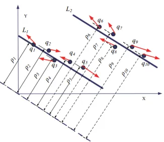
Isolated Point Labeling. After the line detection step, there are some points that cannot be given appropriate labels because their parameters do not belong to any lines. These points are called isolated points. Some isolated points are physically close to and may belong to one line, but the previous θ and ρ based rule cannot assign the point a label because of the threshold. To reassign these points with appropriate labels, we evaluate the distance of the point to the line segment, to judge whether we should assign this isolated point the corresponding line label. The distance of the point to the line segment ( ) defined here is slightly different from the distance of a point to a line. The distance is the minimal distance from the point to any of the points inside the line segment, as shown in Figure 6a. Here, are the distances of three different points to the line segment L in three situations. is located at the left, is located at the right, and the perpendicular foot of is located inside the line segment. If the distance of the point is lower than average point gap, will be assigned to ;

(a) (b)

Figure 6. The reason for using the distance to the line segment.

segment and a smaller value to line segment . If the label of the point is judged by the distance to the line segment rather than to a line, then wrong assignments caused by this situation can be avoided.

Line Stability Descriptor (LSD). In this section, the structural relation of the line is studied and used to improve the line detection results. We assume the following: (1) voting based line detection results are not reliable, but can be used as the seeds of line segments for further refinement process; and (2) the stability of each line is different and can be measured. For example, a line with a greater fitting residual implies poorer line stability and a higher probability of being a wrong result.

We first designed a descriptor, called Line Stability Descriptor (LSD), which has four element to evaluate the stability of each line segment. The four elements are: the length of the line ( ), the geometric regularity ( ), the fitting residual ( ) and the point number ( ). For the difference data units of the four elements, the normalized function for each element is defined to transform the data from various units and sizes into the same unit. Finally, we join the four elements descriptors into one value that can represent the stability of a line segment. The details of the four elements are given below:

Length of Line. _{For the edge of a building, a longer edge line that is detected has a higher} probability of being a correct line segment than a shorter one. This assumption is built on the length of the line element. The value indicates the contribution of the length of the line segment to the stability, as defined below:

(5) Where is the length of the line and is the length threshold. In equation 5, if is longer than , because we thought it was stable enough, the will be given value 1. The value of in this equation defines how long we believe the line is sufficiently stable. In the implementation, is set to be 8 meters empirically.

Geometric Regularity. _{If a line is perpendicular or parallel to other lines, then that means this line} has more chance to be a correctly fitted line. In fact, geometric regularity has a large amount of meaningful information, as discussed by [20,22], which can be applied to augment the line detection, such as a 45 degree intersection, pattern of array, or other regularities. To simplify the processing, we use only perpendicular and parallel relationships as the constraints.

Given a group of line segments L from each building with n + 1 line segments with pairs of parallel OR perpendicular (regular relation) line segments in L, for a line segment in L,

donates that has a regular relation with m other line segments. Then the geometric regularity index ( ) of is defined as in formula 6. In this formula, the value of is defined to evaluate the stability of the whole structure between the line segments. is a threshold to indicate a weak relation of regularity between the line segments in this group. defines how many line segments has regular relation with is sufficiently stable. After several experiments, and are both set to be value of 3 empirically.

Number of Points. _{The number of composed points of a line segment is related to the line} stability. This element is related to the length of the line, but it indicates more information. For example, given a point set with three collinear points but the distances between each two points are large, if we fit them into a line, then the residual of the fitting is zero, and the length of line segment is long, but the line is not stable at all. To avoid this situation, we define this indicator to describe the stability of the line. If denotes the number of points of a line segment, then the value of this indicator is given as in the formula 7. For strongly correlation to the point density of the value of , the threshold for and are established by the smallest length line segment in an

object and the average point gap as and .

(7) Fitting Residual. _{A small residual of fitting implies a stable collinear relation of points. If r is the} residual value of the line fitting, and c is the number of points in the line segment, then the fitting residual indicator value is defined as below:

(8) Similar to the previous indicators, the lateral placement accuracy of the data used in this formula are determined by the data quality. Besides, is defined as the limitation value to exclude the gross error.

Line competition. Based on these four elements, we design a structure sensitive optimization algorithm to adjust the detected line segments by applying a competition process to each line segment. Every point is competed by the close line segments to find the most suitable line segment to which this point belongs. This procedure appears to be competition of points between line segments. Whether a point belongs to a line segment depends on two conditions: 1) How long the distance of the point is to the given line segment is close; 2) There should be no more other suitable (or closer) line segments other than the current one. To make the four elements easily used in the computation, we combine them into one value, which is denoted by S, and it sums the four indexes with difference weights as in equation 9.

(9) Here, are the weights to the corresponding elements. In this paper, we assign the same weight value for these four elements.

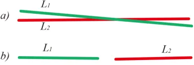
than triple average point gap and the perpendicular distance from line segment to line is lower than one average point gap, two line segments will be merged.

Figure 7. Two situation of line segments merging.

Line Break. _{A line segment L breaks into two short line segments L1 and L2. The line segments} L1 and L2 will take their corresponding points from the original line segment L. The line segments L will disappear because all of the points that belong to L are taken away. As shown in Figure 8, at the beginning, L is composed of a group of collinear points as in Figure 8a. After the hollow point in Figure 8a is taken away as in Figure 8b, the line segment breaks into two line segments, L1 and L2, as shown in Figure 8c. Here, whether one line segment will break into two depends on the condition where the distance between adjacent points from the line segment is greater than triple average point gap.

Figure 8. One line segment breaks into two after some points are taken away.

During the line segment competition, if one line segment takes points from the others, then its parameters will be updated. If the new parameters of this line segment are similar to one neighboring line segment and under the merging condition, then they will be merged into one. In contrast, if the points of one line segment are taken away by other line segments, then the parameters of that line segment will be updated and its stability will also be re-evaluated. If the connectivity between the points in one line segments cannot be maintained, then the line segment will be broken into two or more pieces. During the line segment competition process, there are line segment merging and line segment breaking. In line segment merging, the points of one line segment will be given to another one, and the new line’s parameters will be estimated by all of the points. In Line segment breaking, one line segment will break into pieces according to the distance between the component points. Thus, some of the line segments will disappear after their points are taken away.

Experiments

The building feature line extraction is evaluated by completeness, correctness and quality of the results as [15]. Recall and Precision are used to evaluate the completeness and correctness of each building respectively. The Recall is defined as the ratio between the number of the that correspond to the detected lines and the total number of . The Precision is denoted as the ratio between the number of the detected lines that correspond to and the total number of extracted lines. To evaluate the quality of the extracted features lines, three parameters are given.

Overlap rate is the overlap length in the extracted building, and is the number of extracted lines. is the length of each ground truth line, and is the number of ground truth lines.

(10) Distance error is defined as the average distance between two end points of the extracted line to its matched line from . denotes the length of the extracted line.

(11) Orientation error is the angle between and its matched line from .

(12) Additionally, the extracted line is considered to correspond to if its to matched is not larger than double point gap and its is less than the value of .

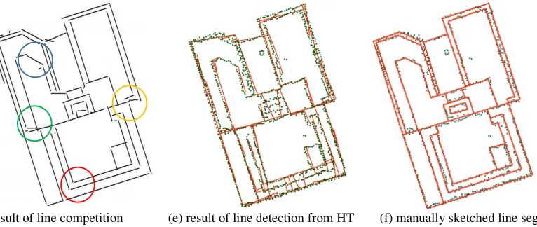
(d) result of line competition (e) result of line detection from HT (f) manually sketched line segments

Figure 9. The line extraction results at each steps. The quality of the extracted lines improves substantially after processing (d) the line competition.

Test I. _{The results of each processing steps are shown in this experiment from the original points} to the final outputs. Figure 9a is the corresponding point clouds colored by height values. The black points in Figure 9a are the step edge points detected by the height deviation of each point and its neighboring points, and we give the value of 2m as the threshold of height deviation as we did in [18]. The value of is given as 1.0 meter empirically for the consideration of 1.0 meter is the smallest line segment we will detect. Figure 9b shows the result of the detected line segments only by the point voting. In this experiment, the distance threshold for the neighboring point search is approximately 2 meters. After the re-assignment of the isolated points, at the corner of the building, the extracted line segments substantially retrieve part of corner points in Figure 9c which corresponds to the increasing of the overlap rate of procedure point voting and reassigning isolated points in Table 1.

Table 1. Comparison of the detection results from our method and the HT.

Recall[%] Precision[%] Overlap[%] Distance[m] Orientation[ ]

points voting 0.942 0.869 0.776 0.183 2.975

isolated points 0.942 0.877 0.850 0.179 2.799

Line competition 0.942 0.917 0.910 0.090 0.650

HT 0.615 0.867 0.879 1.22 3.432

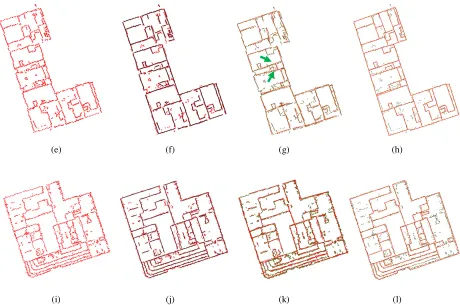
(e) (f) (g) (h)

(i) (j) (k) (l)

Figure 10. Edge points, extracted results of our method and results of HT. (a), (e), (i) are the edge points detected from the Toronto data set. (b), (f), (j) are the line features extracted using our algorithm. (c), (g), (k) are the results of the line

extraction by HT. (d), (h), (l) are the results of the line performed manually.

Compared to Figure 9c, Figure 9d shows those weak line segments that are short, noisy and lack regular relationships lost points continuously. After several iterative steps of competition, some weak line segments disappear and their points are merged into the strong line segments. Figure 9e shows the line detection result by HT. To make the test data be easily processed by the HT algorithm, we interpolate the edge points into a raster image with a resolution according to the density of the point clouds, which is 0.6 meters in our experiment. Then, we use the raster map to estimate the parameters of the feature lines by the Standard Hough Transformation (SHT).

We compared the results of the proposed method and HT with the manually extracted line segments shown as Figure 9f to give a quantified evaluation, and the overall assessment are shown as Table 1. For the test building, our algorithm detected 49 of the edges from 52 manually sketched reference edges. At the same time, the HT algorithm detected 40 of them. From the lower value of Recall, HT detected many long edges, but left the short edges, and HT also considers the relatively higher rate of detecting lengths from the higher overlap rate.

Test II. _{contains 3 typical buildings of increasing edge point number with same data precision and} density as test I. Figure 10 shows the edge points of three buildings, the detected line features using our algorithms, HT algorithm and manual extraction. The edge points are directly detected from the point cloud data (Figure10a, 10e and 10i). Figure10a is a building with a simple structure that is composed by two connected units with several affiliate objects on the roofs. All of the edge lines of this building are orthogonal or parallel (Figure10a). Figure10b shows the extracted line features by our method, overlapping the original edge points. Compared with Figure10b, the results of HT (Figure10c) shows many wrong detections at the corners or noisy parts of the building where the green arrow points.

HT algorithm and our method both have reasonable results for the long and stable edges of this building. However, the HT’s global search strategy generates some over detections at the middle part of the building (where the arrow points). For no line competition processing in HT, the wrong detection results cannot be properly eliminated.

Figure10i is a building that has many detailed line features and noisy clustered points. In Figure10j, even though a large amount of noise exists, our algorithm still gives stable results at the marked area. At the bottom of the building, there is a cluster of noisy points of parallel line segments, and our algorithm does not get influenced, whereas the HT gives many short pieces of line segments.

Using the method of quality evaluation as performed in Test I, the results are shown in table 2. For these three test buildings, our algorithm does not acquire an evident superiority in Recall and Precision over HT algorithm. However, in the item of Distance and Orientation, our propose method has more accurate line segment.

Table 2. Comparison of the detection results from our method and the HT. (Unit: Meter).

Method Recall[%] Precision[%] Overlap[%] Distance[m] Orientation[ ]

Building a Ours 0.805 0.814 0.839 0.192 0.668

HT 0.756 0.754 0.816 0.448 2.724

Building b Ours 0.706 0.855 0.695 0.327 1.539

HT 0.624 0.837 0.630 0.616 3.464

Building c Ours 0.685 0.657 0.735 0.364 0.908

HT 0.663 0.732 0.724 0.598 3.695

Discussions

symmetry and curved axis symmetry detection in the 2D image, [11] defined the regular information in 3D space and presented a method for detecting p, the regularity. These research results can be utilized in understanding the structure of the building and thus can add more constraints and improve the modelling process.

Conclusions

In this paper, we propose a feature line detection algorithm specifically for building objects from airborne LiDAR data. The algorithm attempts to augment the line extraction results with information embedded inside the points and real objects. It deepens the line feature detection algorithm according to the characteristics of the specific goal of building model reconstruction, and utilizes the points’ relationships as well as the line segments structure relationships to polish the extraction results. A large amount of uncertainty in the line detection can be avoided for the structural constraints, and our results show an obvious stability in comparison with the HT method.

However, the edge detection method used in our experiment is suitable for detecting step edge points from airborne LiDAR point clouds, but might not work well in detecting the points of the ridges, especially the intersecting ridges of two roof planes. Of course, we can use other edge detection methods to detect the edge points from the point clouds by algorithms such as the canny algorithm or curvature flow [23,24]. This method also has its limitations for objects that do not have any explicit structural relationships. For some buildings of non-regular geometric shapes and in which the step edges do not have orthogonal or regular relationships, the orthogonal weight of the line optimization will fail. On the hand, this paper did not mention how to combine the extracted line features into a complete building footprint. In fact, the feature lines extracted can be used as inputs for a partition and merge algorithm for building model reconstruction [7].

Acknowledgments

This research was supported by the National Basic Research Program of China (No. 2012CB725300), National Key Technology Support Program of China (No. 2012BAH43F02), National Natural Science Foundation of China No. 41001308 and No. 41071291.

References

[1] Lafarge, F.; Mallet, C. Building large urban environments from unstructured point data. 2011 Ieee International Conference on Computer Vision (Iccv) 2011, 1068-1075.

[2] Maas, H.G.; Vosselman, G. Two algorithms for extracting building models from raw laser altimetry data. ISPRS Journal of Photogrammetry and Remote Sensing 1999, 54, 153-163.

[3] Vosselman, G.; Gorte, B.G.; Sithole, G.; Rabbani, T. Recognising structure in laser scanner point clouds. International archives of photogrammetry, remote sensing and spatial information sciences 2004, 46, 33-38.

[4] Chen, J.; Chen, B. Architectural modeling from sparsely scanned range data. International Journal of Computer Vision 2007, 78, 223-236.

[5] HABIB, A.; ZHAI, R.; KIM, C. Generation of complex polyhedral building models by integrating stereo-aerial imagery and lidar data. American Society for Photogrammetry and Remote Sensing: Bethesda, MD, ETATS-UNIS, 2010; Vol. 76, p 15.

[7] Sohn, G.; Dowman, I. Data fusion of high-resolution satellite imagery and lidar data for automatic building extraction. ISPRS Journal of Photogrammetry and Remote Sensing 2007, 62, 43-63.

[8] Poullis, C. A framework for automatic modeling from point cloud data. Pattern Analysis and Machine Intelligence, IEEE Transactions on 2013, 35, 2563-2575.

[9] Sampath, A.; Shan, J. Building boundary tracing and regularization from airborne lidar point clouds. Photogrammetric Engineering and Remote Sensing 2007, 73, 805-812.

[10] Lee, S.; Liu, Y. Curved glide-reflection symmetry detection. Pattern Analysis and Machine Intelligence, IEEE Transactions on 2012, 34, 266-278.

[11] Pauly, M.; Mitra, N.J.; Wallner, J.; Pottmann, H.; Guibas, L.J. Discovering structural regularity in 3d geometry. ACM Trans Graph 2008, 27.

[12] Hough, P.V. Method and means for recognizing complex patterns. 1962.

[13] Illingworth, J.; Kittler, J. A survey of the hough transform. Computer vision, graphics, and image processing 1988, 44, 87-116.

[14] Burns, J.B.; Hanson, A.R.; Riseman, E.M. Extracting straight lines. Pattern Analysis and Machine Intelligence, IEEE Transactions on 1986, 425-455.

[15] Truong-Hong, L.; Laefer, D.F. Quantitative evaluation strategies for urban 3d model generation from remote sensing data. Computers & Graphics 2015.

[16] Truong-Hong, L.; Laefer, D.F.; Hinks, T.; Carr, H. Combining an angle criterion with voxelization and the flying voxel method in reconstructing building models from lidar data. Computer-Aided Civil and Infrastructure Engineering 2013, 28, 112-129.

[17] Vosselman, G. Building reconstruction using planar faces in very high density height data. International Archives of Photogrammetry and Remote Sensing 1999, 32, 87-94.

[18] Sohn, G.; Huang, X.F.; Tao, V. Using a binary space partitioning tree for reconstructing polyhedral building models from airborne lidar data. Photogrammetric Engineering and Remote Sensing 2008, 74, 1425-1438.

[19] Bartholdi III, J.J.; Goldsman, P. Multiresolution indexing of triangulated irregular networks. Visualization and Computer Graphics, IEEE Transactions on 2004, 10, 484-495.

[20] Vosselman, G.; Dijkman, S. 3d building model reconstruction from point clouds and ground plans. International Archives of Photogrammetry, Remote Sensing and Spatial Information Sciences 2001, 34, 37-44.

[21] O'gorman, F.; Clowes, M. Finding picture edges through collinearity of feature points. Computers, IEEE Transactions on 1976, 100, 449-456.

[22] Ameri, B. Feature based model verification (fbmv): A new concept for hypothesis validation in building reconstruction. International Archives of Photogrammetry and Remote Sensing 2000, 33, 24-35.

[23] Canny, J. A computational approach to edge detection. Pattern Analysis and Machine Intelligence, IEEE Transactions on 1986, PAMI-8, 679-698.