2019 2nd International Conference on Informatics, Control and Automation (ICA 2019) ISBN: 978-1-60595-637-4
Collaborative Representation and Sparsity are Both Indispensable for
Hyperspectral Imagery Classification
Ji-tai A, Shu-cai HUANG, Xiao-fei LI and Yi-dong TANG
*Changle East Road No.1, Xi’an, Shan’xi, China
*Corresponding author
Keywords: Hyperspectral imagery, Classification, Sparse representation, Collaborative representation.
Abstract. As a recently proposed technique, sparse representation based classifier (SRC) has been widely used for hyperspectral imagery classification and detection. The collaborative representation (CR) and the sparse coding are two key points in SRC scheme. More recently, the proposition that which one of them plays a dominant role in SRC scheme has attracted much attention from researchers in fields of image processing, computer vision, and pattern recognition. In this paper, we first discuss why CR or sparsity works and why one of them alone is not sufficient, and then analyze how CR and sparsity interact with each other. Although we focus on how sparsity augments CR, the necessity of CR for sparsity is also illustrated in both pixel-wise model and joint sparsity model. Inspired by the analysis, we indicate that CR is a powerful tool for solving the high-dimensional pattern recognition with small sample in SRC scheme; sparsity augments CR-based classification in stabilizing, making sure unique solution and rejecting outlying samples. In other words, CR and sparsity complement each other and are both indispensible for hyperspectral imagery classification. The experimental results on simulated data and real hyperspectral imagery confirm the conclusion.
Introduction
HYPERSPECTRAL imagery provides a wealthy of spectral information, which spans the visible to infrared spectrum. Different materials usually reflect electromagnetic energy differently at specific wavelengths. This makes it possible to uniquely identify various materials based on their spectral signatures. One of the most important applications of HSI is image classification, where pixels are labeled to one of the classes based on their spectral characteristics and training samples for each class. Various techniques have been developed for HSI classification. Comparing with previous approaches, the support vector machine (SVM) [1] [2] [3] has been proved to be a powerful tool to solve supervised classification problem in remote sensing and performs well. And variations of SVM based algorithms have also been proposed to improve its performance [4] [5].
In a sense, the SRC can be treated as a CR-based classifier (CRC) with sparse constraint. For a better understanding and comparison, we define the general SRC as sparse CRC (SCRC) and the CRC without sparse constraint as dense CRC (DCRC). The main idea of this paper is the roles that CR and sparsity play in CR-based classifier but not algorithm designing. We first extend the analysis in [15], and discuss why CR or sparsity works and why one of them alone is not sufficient. Then, we analyze the interactions between CR and sparsity, and indicate that CR and sparsity complement each other in HSI classification, and neither can work effectively without each other. On one hand, sparsity improves the discriminative power of representation error when too many samples are used or subjects look similar with each other, leading to a robust classification. On the other hand, sparse representation codes a test pixel over an over-completed dictionary. However, HSI classification is a typical high dimensional problem with small sample size, leading to an under-completed dictionary. One of the tools for solving the “lack of samples” problem is CR that takes the samples from all the other classes as the possible samples of each class. In turn again, the CR coding may produce same class-specific residuals for different classes, leading to wrong classification in labeling process. In this case, sparsity can be used to make sure the uniqueness and right classification. Although we focus on how sparsity augments CR in stabilizing, making sure unique solution and rejecting outlying samples, the necessity of CR for sparsity is also illustrated in both pixel-wise model and joint sparsity model. Finally, we evaluate SCRC and DCRC as well as their simultaneous joint visions on a real HSI data set to verify our conclusion.
The rest of the paper is organized as follows. Section II briefly reviews general SRC. Section III analyzes how CR and sparsity interact and augment with each other. Experimental results and discussion on data set are provided in Section IV. Finally, we conclude the paper in Section V.
Sparse Representation Based Classifier
In general SRC scheme, it is assumed that the spectral signatures of pixels belonging to same class approximately lie in the same low-dimensional subspace. Denote sub-dictionary by the data set of training samples of classi B Ni
i
X , whereBis the number of spectral bands. Suppose that we
haveK classes of subjects, hence the structured dictionary
1, 2, ,
B N K
X X X X ,
1
K
i i
N N
isformed from the sub-dictionaries. A given query pixel B
y can be coded overX with sparsity constraint.
0
2 0
ˆ arg min yX s.t K
(1)
where
11; ; ; ;
N
i K
andiis the coding vector associated with classi. The 0-norm regularized minimization problem (1) can be solved by OMP algorithm. Once the coding vector is obtained, the class label ofycan be determined by the minimum reconstruction residual associated with each class wise sub-dictionary
2
1, , ˆ
Class( ) arg min i i i K
y y X (2)
where i1, 2, ,Kis the class index.
Collaborative Representation and Sparsity Constraint
As mentioned in the previous section, CR and sparsity constraint are two key points in the coding process of SRC. In this section, concerning how CR and sparsity interact with each other in SRC scheme, we focus on how sparsity augments CR, and also illustrate the necessity of CR for sparsity.
Sparsity is Necessary for Robustness
fact in HIS scene), sub-dictionaryXiand sub-dictionaryXjare not incoherent but can be highly
correlated i.e.Xj Xi. Without regularization term, the coding vectors of yby classiand class j,
i
αandαj, can be calculated by least square method. Letei y Xiαiandej y Xjαj. Suppose
that m n
i j
X , X , andis small such that
s i
F
i F l i
X
X X
(3)
where l Xi ands Xi are respectively the largest and smallest eigenvalues ofXi. Then, we can
get the relationship betweeneiandejas follows
22
2 2
1 min 1,
j i
i m n
e e
X
y (4)
where 2 Xi is the 2-norm conditional number ofXi. We can see from (4) that ifis small, the
distance betweeneiandejcan be very small. This makes the classification so unstable that even a
small disturbance can result in a wrong classification. Furthermore, with enough training samples for each class, we can useXjto representywell even whenydoesn’t belong to class j. In other
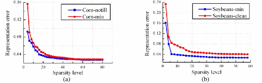
words, the discriminative power of the representation error will reduce if too many samples are used or subjects look similar with each other. To illustrate the observation, we respectively use training samples from Corn-notill and Corn-min in Indian Pines image data set to represent a given Corn-notill sample, and use samples from Soybeans-min and Soybean-clean to represent a given Soybeans-min training sample under different sparsity levels. The curves of representation error versus the sparsity level are drawn in Fig. 1. We can see From Fig. 1 that when the sparsity level is low, both of the right class and wrong class have relatively big error. And the representation error decreases with the sparsity level and tends to saturate as sparsity level reaches a certain value. However, the discriminative power of the representation error reduces if sparsity is too high.
[image:3.595.92.509.461.593.2](a) (b)
Figure 1. The curve of representation error versus the sparsity level.
As a result, the robustness of classification can be enhanced by imposing some sparsity constraint on coding vector. If ybelongs to classi, it is more likely that only a few samples inXican
representywith a good accuracy, while more samples inXjare required to representywith nearly
same accuracy. Hence, under a certain sparsity, the representation error ofybyXiwill be obviously
lower than that byXj, leading to an enhanced discriminative power of representation error. This is exactly the fundamental mechanism in which SRC works.
Sparsity Needs CR
pixel. Unfortunately, HSI classification is a typical high dimensional problem with small sample size, generally leading to an under-completed sub-dictionaryXi. If we use the under-completeXito
representy, the representation error can be large, even whenyis from classi. In SRC, this “lack of
sample” problem is solved by taking the training samples from all the other classes as the possible samples of each class, i.e. collaborative representation. The reason is that samples of different classes share similarities; hence some samples from class jmay be very helpful to represent the query pixel from classi. To understand the working mechanism of CR-based classification, we define the matrix X = X , X ,
1 2 , XK
as the dictionary of all samples, and write the subspacespanned by the columns of X as . In SCRC scheme, it codes the query pixelyover the dictionaryXwith 0-norm constraint, and then identifiesyindividually. When we ignore the 0-norm
constraint in (1), the representation becomes a least square problem 2 2
ˆarg min yX
. Then the
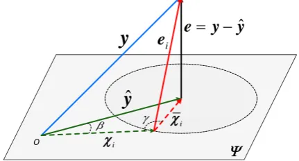
representation y = Xαˆ is actually the perpendicular projection of y onto , and Fig. 2 shows geometrically illustration of the representation.
y
ˆ
y
ˆ [image:4.595.189.405.281.397.2]e y y i e i i O
Figure 2. Geometric illustration of the representation ofyover X.
As shown in Fig. 2, without loss of generality, we can decomposeˆyinto two components
ˆ i i
y (5)
where iXiˆi is the representation associate with class i, and
1 ˆ
K
i j i j j
j
X is the sum of
representation associate with all the other classes except classi. The representation error of each class ei yXiˆi 22 is used for classification. It can be derived that
2 2
2 2
ˆ ˆ ˆ
i i i
e yy + yX
(6)
Actually, it is the term * 2
2
ˆ ˆ
i i i
e yX that works for classification because yyˆ 22 is a constant for all classes. Based on sine theorem, we can readily have
2
2ˆ ˆ ˆ
sin sin
i i
y y X
(7) where is the angle between yˆ andi, and is the angle between i and i. Finally the
representation error can be represented as
2 2 2 * 2
i 2 2
ˆ sin ˆ ˆ = sin i i e
y
y X
(8) In (8), the ratio 2 2
they also believe that it is not necessary to use this strong 0-norm whose effects can be replaced by 2-norm. The objective of dense collaborative representation is to allow all the training samples to participate in the representation ofy. As a result, the objective function of collaborative representation with 2-norm regularization is formulated as
2 2
2 2
ˆarg min yX
(9) where is a regularization parameter. Taking derivative with regard toand setting the resultant equation to zero yields
1ˆ T T
X X I X y
(10) Once the coding vector of the representation is obtained, the label ofycan be determined in the same way as SRC in (2).
Why CR Needs Sparsity in Turn
According to Zhang et al. [1], the ratio 2 2
sin sin is powerful for classification. However, for ,
0, 2
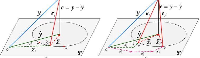
, there is no unique minimum for the given squared ratio in (8). As shown in Fig. 3(a), any vector starting fromoand ending at a point on broken line circle (e.g.p q, ), i.e., representation associate with other class, will have the same *i
e asi . This will finally result in a wrong
classification. This fact is obviously ignored by Zhang et al [1]. That is, the sparsity constraint is not only used to stabilize the least square solution, but to make sure the uniqueness of the minimum for the given squared ratio in (8). As shown in Fig. 3(b), iis composed of 1
i
x and 2
i
x , atoms fromXi;
andjis composed of
1
j
x , 2
j
x and 3
j
x , atoms fromXj. Although the class-specific residuals are equal,
we can still label the query pixel as classisinceirequires lesser number of atoms to produce the same class-specific residual. Hence, the performance of CR-based classification is augmented by sparsity constraint.
y
ˆ
y
ˆ e y y
i e i i p q O (a) (b)
y
ˆ
y
ˆ e y y
i e j i p q O j e 1 i x 2 i x 2 j x 1 j
[image:5.595.109.488.469.580.2]x x3j
Figure 3. Geometric illustration of the working mechanism of CR-based classification.
In the previous subsection, the number of the components, i.e. sparsity level, is used for pixel-wise classification when the class-specific residuals have equal length. How can sparsity make sure the uniqueness when class-specific residuals and sparsity level forXiandXjare both
number of components. Consequently, the classification will be inaccurate no matter the error or the sparsity or both of them are used for decision making. However, since the sparse vectors associated withy1andy2share a common sparsity support, the components used to represent y1, i.e. 1
i
x paired
with 2
i
x and 1
j
x paired with 2
j
x , also must be used to representy2, just with different weight fromy1. In this case, although it is not possible to use the representation of y1 for classification, the class-specific residuals fory2(εiandεj) are most likely no longer equal and the fact can be used for
classification. Intuitively, i(not j) represents the correct class of the test pixel since components from classiproduce a smaller class-specific error fory2. Hence, cooperating with spatial correlation, the sparsity constraint further makes sure the uniqueness and improves the classification performance. The DCRC and SCRC in JSM are respectively denoted as simultaneous DCRC (SDCRC) and simultaneous SCRC (SSCRC).
1 y
i e
1
p q1
O x2i 2
j x
1
j
x
2
p O1
O2
2
q
2 y
2
ˆ
y
1
ˆ y
1
i x
j e
j
i
[image:6.595.186.409.246.368.2]
Figure 4. Geometric illustration of the working mechanism of jointly sparse representation.
Considering the spatial correlation, the neighboring pixels are simultaneously represented in collaborative representation. Without sparsity constraint (i.e., dense CR), the solution formin Y X 22 2Fis essentially computed column by column. In this case, it just focuses on
jointly calculating the total residuals from all the neighboring pixels, and then uses the total residuals for labeling. In other words, dense CR in JSM wastes the spatial correlation information during coding step. Different from dense CR, the sparse CR takes use of spatial correlation during both coding step and labeling step. Hence, the sparsity constraint augments joint collaborative representation on the utilization of spatial information.
0 2 ˆ arg min s.t yX
(11) where is the error tolerance. The above problem can also be solved by OMP algorithm.
To support our argument, we choose 5 classes of subjects from AVIRIS San Diego, CA, USA as valid, and randomly select 81 samples per class for training. A synthetic data set, 64×64 pixels in size, is constructed of an invalid (denote by Class 0) and the 5 classes of valid samples (denote by Class 1, 2, 3, 4, and 5). Considering the spectral mixture and noise, the spectral signatures are mixed with a background spectrum with abundance of 0.6, and Gaussian noise is then added to achieve a 30:1 signal-to-noise ratio. Then a valid and an invalid pixel are respectively represented by sparse CR (SCR) and dense CR (DCR) under same error level. Fig. 5 shows the distribution of coefficients. We see from Fig. 5 (a) and (b) that, the coefficients of valid pixel by SCR concentrate on first 81 samples (9 out of 21) while the coefficients of invalid pixel nearly spread uniformly across the entire training set (4, 6, 3, 4 and 5 nonzero entries drop into corresponding subjects respectively). Thus, we can distinguish valid pixel from invalid pixel with the distribution of coefficients. However, we see from Fig. 5 (c) and (d) that, the coefficients of valid and invalid samples by DCR both spread widely across the 405 training samples. In this case, the distribution of coefficients cannot be used for query pixel validation in DCR scheme.
(a) (b)
[image:7.595.137.466.303.516.2](c) (d)
Figure 5. Distribution of coefficients of (a) valid pixel by SCR, (b) invalid pixel by SCR, (c) valid pixel by DCR, (d) invalid pixel by DCR.
Experiments and Results
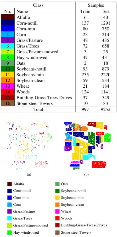
The data set in this paper is the Indian Pines image, and we download the MATLAB data files for experiments (The files can be found on the Group de Intelligence Computational at http://www.ehu.eus/ccwintco/uploads/2/22/Indian_pines.mat.). It was acquired by Airborne Visible/Infrared Imaging Spectrometer (AVIRIS), which generates 220 bands across the spectral range 0.2 to 2.4m. 20 noisy bands are removed due to water absorption bands before classification. This image is 145×145 pixels in size with a spatial resolution of 20 m/pixel, and contains 16 ground-truth classes. For each class, we randomly choose around 10% of the labeled pixels for constructing the dictionary and use the remaining 90% pixels for testing, as shown in Table I and Fig. 6. In our experiments, overall accuracy (OA) and average accuracy (AA) are used to evaluate the classification performance. The OA is the ratio between correctly classified test samples and the total number of test samples, the AA is the mean of the 16 class accuracies.
Table 1. Indian Pines Ground-Truth Classes and Train/Test Sets.
Class Samples
No. Name Train Test
1 Alfalfa 6 40
2 Corn-notill 137 1291
3 Corn-min 80 750
4 Corn 23 214
5 Grass/Pasture 48 435
6 Grass/Trees 72 658
7 Grass/Pasture-mowed 3 25
8 Hay-windrowed 47 431
9 Oats 2 18
10 Soybeans-notill 93 879
11 Soybeans-min 235 2220
12 Soybean-clean 59 534
13 Wheat 21 184
14 Woods 124 1141
15 Building-Grass-Trees-Drives 37 349
16 Stone-steel Towers 10 83
Total 997 9252
Alfalfa
Corn-notill Corn-min Corn Grass/Pasture Grass/Trees Grass/Pasture-mowed Hay-windrowed
Oats
Soybeans-notill Soybeans-min Soybean-clean Wheat Woods
Building-Grass-Trees-Drives Stone-steel Towers
(a) (b)
Figure 6. (a) Training and (b) test sets for the Indian Pines image.
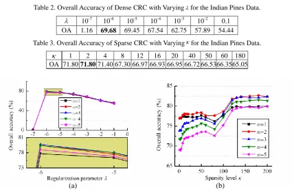
Parameter Analysis: For optimal parameter selection, we compute the OA of DCRC with varying regularization parameterranging from 10−7 to 0.1, as well as the OA of SCRC with varying sparsity levelranging from 1 to 40, as listed in Table 2 and Table 3. One can see from Table 2 and Table 3 that for the pixel-wise CR model, 6
10
leads to the greatest OA for DCRC, and
2
leads to the greatest OA for SCRC. Similarly, we also compute the OA of SDCRC with varying neighbor sizeand, as well as the OA of the SSCRC with varying neighbor sizeand sparsity level, as shown in Fig. 7. One can see from Fig. 7 (a) that 6
10
leads to the greatest OA at all neighbor
sizes for SDCRC in the JSM. For a fixed, the performance of SDCRC changes a little with neighbor size. For SSCRC, as shown in Fig.7 (b), 2leads to the greatest OA at all sparsity levels. For a fixed, the performance of SSCRC generally has two local highest points and tends to saturate as sparsity levelreaches 140–200. As a result, we fix106and
3
Table 2. Overall Accuracy of Dense CRC with Varyingfor the Indian Pines Data.
10-7 10-6 10-5 10-4 10-3 10-2 0.1 OA 1.16 69.68 69.45 67.54 62.75 57.89 54.44
Table 3. Overall Accuracy of Sparse CRC with Varyingfor the Indian Pines Data.
1 2 4 8 12 16 20 40 50 60 180
OA 71.80 71.80 71.40 67.30 66.97 66.93 66.95 66.72 66.53 66.35 65.05
(b) (a)
Figure 7. Parameter analysis. OA values of (a) SDCRC at differentand, (b) SSCRC at differentand.
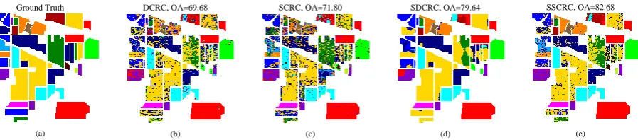
[image:9.595.192.403.509.744.2]Classification performance: With optimized parameters, Table 4 shows classification accuracy for each single class, OA, and AA. Fig. 8 shows the ground-truth and classification maps. Fig. 8(b) and (c) respectively show the classification maps of DCRC and SCRC in pixel-wise model, while Fig. 8(d) and (e) respectively show the classification maps of SDCRC and SSCRC in JSM. We can clearly see that sparsity constraint has significantly improved the classification performance whether or not the spatial correlation is incorporated. The SSCRC outperforms the other three classifiers, with greatest OA and AA. It is sparsity constraint that further improves the classification accuracy in cooperation with spatial correlation, as mentioned in section III.
Table 4. Classification Accuracy (%) for AVIRIS Indian Pines.
Class DCRC SCRC SDCRC SSCRC
1 4.35 41.30 0 78.26
2 67.16 52.80 77.87 75.84 3 44.82 60.48 60.84 58.19 4 12.24 46.84 5.91 64.56 5 66.67 82.40 79.92 91.10 6 93.56 92.74 99.73 99.45
7 0 92.86 0 92.86
8 97.28 94.56 100 100
9 0 40.00 0 10
10 43.00 68.52 41.15 57.00 11 79.06 73.40 96.99 89.53 12 48.23 50.93 69.81 78.08 13 97.56 94.63 98.54 97.56
14 98.42 94.39 100 99.76
15 37.05 43.52 47.67 71.76
16 82.80 92.47 100 100
(e) SDCRC, OA=79.64
Ground Truth DCRC, OA=69.68 SCRC, OA=71.80
(a) (b) (c) (d)
[image:10.595.79.528.70.169.2]SSCRC, OA=82.68
Figure 8. Ground-truth and classification maps with OA for the Indian Pines image.
Conclusion
The main idea of this paper is the intertwined roles that CR and sparsity play in CR-based classifier but not the algorithms design. And in contrast to the existing notion about which one is more important, this paper tried to reveal that the CR and sparsity are both indispensable for classification. Both of them play an explicit role in CR-based classification for hyperspectral imagery. No matter in pixel-wise model or JSM, the CR is crucial for sparse representation when lacking training sample, while the sparsity augments CR-based classification in several ways. The experimental results clearly demonstrate the conclusion.
Acknowledgement
This work was supported by the National Natural Science Foundation of China under Grant 61273275 and Aeronautical Science Foundation of China under Grant 20130196004.
References
[1] F. Melgani and L. Bruzzone, “Classification of hyperspectral remote sensing images with support vector machines”, IEEE Trans. Geosci. Remote Sens., Vol. 42, No. 8, pp. 1778–1790, 2004.
[2] B. E. Boser, I. M. Guyon, and V. N. Vapnik, “A training algorithm for optimal margin classifiers”, in Proc. 5th Annu. Workshop Comput. Learn. Theory, 1992, pp. 144–152.
[3] J. A. Gualtieri and R. F. Cromp, “Support vector machines for hyperspectral remote sensing classification”, in Proc. SPIE 27th AIPR Workshop: Adv. Comput.-Assist. Recognit., Washington, DC, Oct. 1998, Vol.3584, pp. 221–232.
[4] G. Camps-Valls and L. Bruzzone, “Kernel-based methods for hyperspectral image classification”, IEEE Trans. Geosci. Remote Sens., Vol. 43, No. 6, pp. 1351–1362, 2005.
[5] Bruzzone, M. Chi, and M. Marconcini, “A novel transductive SVM for the semi-supervised classification of remote sensing images”, IEEE Trans. Geosci. Remote Sens., Vol. 44, No. 11, pp. 3363–3373, 2006.
[6] J. Wright, A. Y. Yang, A. Ganesh, S. Sastry, and Y. Ma, “Robust face recognition via sparse representation”, IEEE Trans. Pattern Anal. Mach. Intell, Vol. 31, No. 2, pp. 210–227, 2009.
[7] A. M. Bruckstein, D. L. Donoho, and M. Elad, “From sparse solutions of systems of equations to sparse modeling of signals and images,” SIAM Rev., Vol. 51, No. 1, pp. 34–81, 2009.
[8] M. Elad, Sparse and Redundant Representations: From Theory to Applications in Signal and Image Processing. New York: Springer-Verlag, 2010.
[9] M. Elad, M. A. T. Figueiredo, and Y. Ma, “On the role of sparse and redundant representations in image processing,” Proc. IEEE, Vol. 98, No. 6, pp. 972–982, Jun. 2010.
[11] J. Wright, Y. Ma, J. Mairal, G. Sapiro, T. Huang, and S. Yan, “Sparse representation for computer vision and pattern recognition,” Proc. IEEE ,Vol. 98, No. 6, pp. 1031–1044, Jun. 2010.
[12] A. M. Bruckstein, D. L. Donoho, and M. Elad, “From sparse solutions of systems of equations to sparse modeling of signals and images,” SIAM Rev., Vol. 51, No. 1, pp. 34–81, 2009.
[13] Y. Xu, D. Zhang, J. Yang, and J.-Y. Yang, “A two-phase test sample sparse representation method for use with face recognition,” IEEE Trans. Circuits Syst. Video Technol., Vol. 21, No. 9, pp. 1255–1262, Sep. 2011.
[14] Zongze Yuan, Hao Sun, Kefeng Ji, et al, “Local sparsity divergence for hyperspectral anomaly detection,” IEEE Geosci. Remote Sens Lett, Vol. 11, No. 10, pp. 1697–1701, 2014.