Identification of Dangerous Lines Based on Power Flow Transfer

2018 International Conference on Computer, Communications and Mechatronics Engineering (CCME 2018) ISBN: 978-1-60595-611-4

Identification of Dangerous Lines Based on Power Flow Transfer

Ruo-fa CHENG and Xin FU

Nanchang Hangkong University, No.696, Fenghe South Avenue, Nanchang City, Jiangxi 330063, China

*Corresponding author

Keywords: Reactance weighting matrix, Line tripping distribution factor, Power flow stability index, Power margin, Shortest path searching.

Abstract.In order to avoid grid cascading trip caused by power flow transfer, a search method for key lines based on power flow transfer when single line disconnection is proposed. Searching for several shortest paths between the end points of the removed line base on reactance weighting matrix and branches of all paths form the initial branch set. Then define the power flow stability index to filter the initial branch set to determine the key lines with overload risk. The simulation example shows that the proposed method can quickly and accurately find the dangerous line when power flow transfer, and overcome the shortcomings of the formula complexity of the previous method and the large amount of calculation, which saves time for the subsequent power flow control of circuit network. The proposed method was verified in the IEEE30 node system.

Introduction

When a line in power grid is removed, the power flow on the line will be transferred to other lines, which may lead other lines to overload easily. And the backup protection mechanism will disconnect the overload line, and then result a chain trip in the power grid. If high risk line can be quickly identified when power flow transfer happened and the corresponding control measures are taken to eliminate the overload, the chain trip accident can be effectively prevented.

At present, there are lots of researches on the key lines of power flow transfer when single line is removed. In reference [1], the method of searching for the shortest path by using the reactance of branch and load rate reciprocal as matrix weights may select extra lines. In reference [2], the search method of parallel line with equal voltage phase is complicated and computationally intensive when identify the key lines. In reference [3], the former K paths are used to search for high risk lines, but only the value of the power flow transfer factor is considered when selecting the key lines, and it is not determined whether the power transfer will cause the branch overload.

To the shortcomings of existing methods, a search method for the key lines based on power flow transfer when single line disconnect is proposed. Searching for the former K shortest paths based on reactance weighting matrix between the two end points of the disconnected line to determine the initial set of power flow transfer lines. Then the branch power flow stability index is defined by the line tripping distribution factor and the safety margin of the branch would be used to filter the key lines out.

Searching of Power Flow Transfer Lines

Reactance Weighting Matrix

In an ultra-high voltage power grid, the resistance of the line is much smaller than the reactance. Therefore, the reactance value of the line is used as the weight of the node association matrix. The formation of the reactance weighting matrix B is as shown in (1):

𝐵 = {𝑥𝑖𝑗 𝐴(𝑖, 𝑗) = 1

𝑥_𝑖𝑗 is the reactance value of the branch 𝑖 - 𝑗; the matrix A is the adjacency matrix of the power grid system, and 𝐴(𝑖, 𝑗)=1 represents the node 𝑖 and the node 𝑗 are connected by a line.

Path Searching of Power Flow Transfer

Analysis of Characteristics of Power Flow Transfer

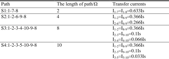
A diagram of power grid is shown in figure 1，and the power flow transfer is analysed after the branch 1-8 is removed. There are four paths between the two end points of the removal branch. The impedance of each branch is shown in figure 1. From the data in figure 1, the current of each branch can be calculated as shown in table 1.

Figure 1. Diagram of power flow analysis.

Table 1. Transfer current of the branch in each path in Figure 1.

Path The length of path/Ω Transfer currents

S1:1-7-8 2 I1-7=I1-8=0.633Is

S2:1-2-6-9-8 4 I1-2=I8-9=0.366Is

I2-6=I6-9=0.266Is

S3:1-2-3-4-10-9-8 8 I1-2=I8-9=0.366Is

I2-3=I9-10=0.1Is I3-4=I4-10=0.066Is

S4:1-2-3-5-10-9-8 10 I1-2=I8-9=0.366Is

I2-3=I9-10=0.1Is I3-5=I5-10=0.033Is

It can be seen from the data in table 1 that the shortest path S1 is composed of the branches 1-7 and 1-8, and the transfer currents on the two branches account for 63.3% of the total transfer current; the currents of branches in the second short path S2 are also large; the currents on branch 1-2 and branch 8-9 on path S3 are also large, and the transfer currents of other branches are small; except the branch 1-2 and the branch 8-9 are larger, the currents of the other branches are very small on path S4. By further analysis, it can be found that both branches 1-2 and 8-9 having a large transfer current in the path S3 and the path S4 are already present in the path S2. Therefore, in this example, the set of branches that are most affected by the power flow transfer can be determined by searching the former two paths. By analogy, for the general grid research, it is possible to determine the set of branches that are more affected by the transferred power flow by searching for several paths with the smallest total impedance value.

Top K Shortest Path Search

Owing to reactance value of the line in the high-voltage transmission network is much larger than its corresponding impedance value. Therefore, in the calculation, using reactance value instead of impedance value [5]. When the topology of the power grid is known, it is known from the graph theory that the grid structure can be abstracted into a graph G (V, E), where V represents the set of bus in the grid and E represents the set of lines between the buses.

The graph G0 (V0, E0) obtained by the abstraction of the transmission network in this paper is an

undirected graph. The weight of E0 is the reactance value of the corresponding line, and V0 is the set

get it by using the improved algorithm based on Dijkstra algorithm [5, 9]. The selection principle of K value satisfies the constraint condition in equation (2) [3].

{ K = max (i|

𝐷𝑖

𝐷1 ≤ M)

𝐾 ≤ 𝑁 (2) 𝐷𝑖 is the length of ith shortest path between the endpoints of the removal line; M is the threshold

of the ratio of the length of the path; N is the upper limit of the number of selected paths.

From the analysis of the correlation data of the branch currents of each branch in table 1, it can be known that the longer of the path, the smaller current of the branch. In the example analysis in section 1.2.1, the length of the first path is 2 Ω, the length of the second path is twice the first, and the length of the third path is 4 times of the first, the length of the fourth path is 5 times the length of the first path. The first path and the second path occupy most of the transfer current, and the transfer currents occupied by the third and fourth paths are very small. So in the calculation of this paper, the value of M is 2; and in case the calculation time from being too long, the value of N is 2.

Line Tripping Distribution Factor

In ground state, after a branch of the power grid is removed, the power flow on the branch will be totally transferred to other branches under the assumption that the active power injection of each node is unchanged. The line tripping distribution factor of the power grid is defined as shown in (3).

𝑇_𝑖 =𝛥𝑃𝑖

𝑃𝑘 (3)

𝑇𝑖 is the line tripping distribution factor of branch 𝑖; 𝛥𝑃𝑖 is the power flow variation of branch 𝑖

after branch 𝑘 is removed; 𝑃_𝑘 is the line power flow before branch 𝑘 is removed.

When (3) is used to determine the branch flow distribution factor of the relevant line, it requires multiple times calculation of power flow and the more time will be costed on it. In order to reduce unnecessary power flow calculation, this paper uses (4) to calculate the line tripping distribution factor of the relevant branch.

𝑇_𝑘−𝑙 = 𝑋𝑘−𝑙⁄𝑥𝑘

1−𝑋𝑙−𝑙 _𝑥 𝑙

⁄ (4)

𝑇_𝑘−𝑙 is the line tripping distribution factor of the branch 𝑘 to the branch 𝑙; 𝑋_𝑘−𝑙 is the mutual impedance between the branch 𝑘 and the branch 𝑙; 𝑋_𝑙−𝑙 is the branch 𝑙 self-impedance; 𝑥_𝑙 and 𝑥_𝑘 are the impedance values of line 𝑙 and line 𝑘 in the impedance matrix of the power grid.

The solution of the mutual impedance between the lines and the self-impedance of the removed line are as follows:

1) Using DC power flow method to calculate the voltage phase of each point, as shown in (5). The active power flow in the power grid always flows from the high voltage phase region to the low voltage phase region [6], so the direction of power flow of each branch in the power grid can be determined by the voltage phase of each point. Therefore, the node-branch correlation matrix M is obtained.

Ɵ = B−1_{· P (5)}

P is the column vector of the active power injected into each node; B is the N-order node admittance matrix; Ɵ is the voltage phase angle column vector of each node.

2) The further derivation by known node-branch association matrix as follows:

𝜇_𝑙 = 𝑋 · 𝑀_𝑙 (6)

𝑋_𝑘−𝑙 = 𝑀_𝑘𝑇_{· 𝜇}

𝑀𝑙 is the node-branch correlation vector of branch 𝑙; 𝑋 is the node impedance matrix of the

power network, which is an inverse matrix with the node admittance matrix; 𝑀_𝑘𝑇 is the transposition of node-branch correlation vector of the branch 𝑘.

Using (4) to calculate the line tripping distribution factor of each branch, the calculation of the power flow of power grid just only once and can be known from the specific calculation process that line tripping distribution factor of branch is independent of the value of power flow of each branch, only related with structure parameters of power grid and direction of branch power flow.

The Determination of Power Flow Stability Index

The power flow stability index of the line is used to measure the difficulty of overload of the line. In this paper, it is used to distinguish the dangerous line when power flow happens.

The Safety Margin of Line

When the power grid system is in normal operation, the active power flows of different lines differ greatly and the maximum transmission power of different lines is also different. The maximum active transmission power is limited by the thermal stability power and the minimum transmission power corresponding to the backup protection setting value. The minimum value of above two values will be selected as the maximum active transmission power. Therefore, the safety margin of active power flow of line 𝑙_𝑖𝑗 is defined as (8).

𝛥𝑃_𝑖𝑗′ = 𝑃𝑖𝑗𝑚𝑎𝑥− 𝑃𝑖𝑗 (8)

𝑃𝑖𝑗𝑚𝑎𝑥 is the maximum active transmission power of line 𝑙𝑖𝑗; 𝑃𝑖𝑗 is the active power of line 𝑙𝑖𝑗.

Power Flow Stability Index

The determination of the power flow stability index combines the power flow safety margin of the line with the line tripping distribution factor of the line, and its specific expression is shown in (9) and (10).

𝑅𝑘−𝑙 = 𝛥𝑃𝑘

′

𝑇𝑘−𝑙 (9)

𝑆𝑘−𝑙 = 𝑅𝑘−𝑙⁄_{𝑃𝑙𝑚𝑎𝑥} = 𝛥𝑃𝑘

′

𝑇𝑘−𝑙·𝑃𝑙𝑚𝑎𝑥 (10)

𝑆_𝑘−𝑙 is the power flow stability index of line 𝑘 when branch 𝑙 is removed; 𝑇_𝑘−𝑙 is the line tripping distribution factor of line 𝑘 when branch 𝑙 is disconnected; 𝛥𝑃_𝑘′ is the active power safety margin of the branch k; 𝑃_{𝑙𝑚𝑎𝑥} is the maximum active transmission power of the breaking branch; 𝑅_𝑘−𝑙 is expressed to ensure that the branch 𝑘 does not overload, the maximum power of line 𝑙 is allowed before the removal.

The specific meaning of the power flow stability index defined in (10) is expressed as follows: when the line 𝑙 is disconnected, if the line 𝑘 is supposed to exceed limit, the ratio of the power flow of line 𝑙 before the disconnection to the maximum active transmission power 𝑊_𝑙 is at least to reach the value obtained by (11), that is, when the power flow 𝑃_𝑙 of the line 𝑙 satisfy (12) before removed, the line 𝑘 will exceed the limit.

𝑊_𝑙 = 𝑃𝑙

𝑃𝑙𝑚𝑎𝑥 (11)

𝑊_𝑙 ≥ 𝑆_𝑘−𝑙 = 𝛥𝑃𝑘′

𝑇𝑘−𝑙·𝑃𝑙𝑚𝑎𝑥 (12)

Through analysing (10) can be obtained that the smaller of 𝑆𝑘−𝑙, the greater risk of line 𝑘 to

k is relatively safe. Therefore, when using the power flow stability index to screen the key line, the line that meets the above conditions will not be considered.

Example Simulation

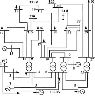
The method proposed in this paper is verified in the IEEE30 node system. The wiring diagram of the IEEE30 node system is shown in figure 2. According to power flow distribution under normal operating conditions, it is simulated by removing several branches. The simulation results are shown in table 2 and table 3.

Figure 2. The wiring diagram of the IEEE30 node system.

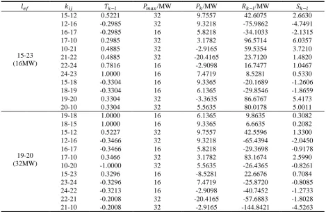
In table 3, 𝑙_𝑒𝑓 represents the removed line, where the value in parentheses is the maximum active transmission power of the line; 𝑘_𝑖𝑗 is the line in the set of the paths that are selected; 𝑇_𝑘−𝑙 is the breaking distribution factor of each line in the branch set after the branch is disconnected.; 𝑃_𝑚𝑎𝑥 indicates the maximum active transmission power of each branch; 𝑃_𝑘 indicates the active power of each branch before the power flow transfer happens; 𝑅_𝑘−𝑙 is expressed to ensure that the branch 𝑘 does not exceed limit, the maximum power of line 𝑙 is allowed before disconnection of line 𝑙𝑒𝑓;

𝑆𝑘−𝑙 indicates the power flow stability index of each line.

Table 2. The results of top K shortest paths when single line disconnected.

Breaking line Top K shortest paths Path length

15-23 15-12-16-17-10-21-22-24-23 1.1400

15-18-19-20-10-21-22-24-23 1.1700

19-20 19-18-15-12-16-17-10-20 1.1600

Table 3. The simulation results of each line when single line disconnected.

𝑙𝑒𝑓 𝑘𝑖𝑗 𝑇𝑘−𝑙 𝑃𝑚𝑎𝑥/MW 𝑃𝑘/MW 𝑅𝑘−𝑙/MW 𝑆𝑘−𝑙

15-23 (16MW)

15-12 0.5221 32 9.7557 42.6075 2.6630

12-16 -0.2985 32 9.3218 -75.9862 -4.7491

16-17 -0.2985 16 5.8218 -34.1033 -2.1315

17-10 0.2985 32 3.1782 96.5714 6.0357

10-21 0.4885 32 -2.9165 59.5354 3.7210

21-22 0.4885 32 -20.4165 23.7120 1.4820

22-24 0.7816 16 -2.9098 16.7477 1.0467

24-23 1.0000 16 7.4719 8.5281 0.5330

15-18 -0.3304 16 9.3365 -20.1689 -1.2606

18-19 -0.3304 16 6.1365 -29.8546 -1.8659

19-20 0.3304 32 -3.3635 86.6767 5.4173

20-10 0.3304 32 5.5635 80.0178 5.0011

19-20 (32MW)

19-18 1.0000 16 6.1365 9.8635 0.3082

18-15 1.0000 16 9.3365 6.6635 0.2082

15-12 0.5227 32 9.7557 42.5596 1.3300

12-16 -0.3466 32 9.3218 -65.4394 -2.0450

16-17 -0.3466 16 5.8218 -29.3698 -0.9178

17-10 0.3466 32 3.1782 83.1674 2.5990

10-20 -1.0000 32 5.5635 -26.4365 -0.8261

15-23 0.3296 16 -8.5281 22.6676 0.7084

23-24 -0.3296 16 7.4719 -25.8720 -0.8085

24-22 -0.3213 16 -2.9098 -40.7452 -1.2733

22-21 -0.2008 32 -20.4165 -57.6883 -1.8028

21-10 -0.2008 32 -2.9165 -144.8421 -4.5263

The analysis of simulation results as follows:

It can be seen from table 1 and table 2 that searching the top K shortest path effectively avoids the lack of key lines, and more accurately discovers the dangerous line. Because the line disconnection may be caused by a natural disaster or crossing current limit, when the power flow exceeds the limit, the line's backup protection device will immediately cut off the line. At this time, the power value is near the maximum transmission power before the line is cut off. For lines 15-23 and 19-20, the values are 16 MW and 32MW. At this time, the power flow index of each branch is 1 when they are removed. Therefore, when the reason of removal is unknown, the disconnection of line15-23 will cause the lines 24-23 to have the risk of over-current limit; When 19-20 is removed, the lines 19-18 and 18-15 is easy to exceed limit, so the two lines are considered as dangerous lines of power flow transfer.

The power flow stability index is defined by the line tripping distribution factor combined with the tidal current safety margin of the line, not only the power flow transfer dangerous lines are not missed, but the power flow calculation is not repeated, the calculation time is less, and correspondingly the algorithm of this paper is faster. In the actual power grid, the number of shortest paths can be flexibly selected according to the actual structural parameters of the power grid system.

Conclusion

Acknowledgement

This work is sponsored by the National Natural Science Foundation of China 51567019.

References

[1] Shen Ruihan, Liu Dichen,et al. Weighted network model based recognition of dangerous lines under power flow transferring, J. Power System Technology, 36(05)245-250, 2012.

[2] Xu Yan, Zhi jing. Quick search for power transfer dangerous lines when multiple branches are disconnected at the same time, J. Journal of Power System and Automation, 29(04)36-42, 2017.

[3] Miao Shihong, et al. A fast recognition method of transmission section based on cut-vertex and path search, J. Automation of Electric Power Systems, 38(02)39-45, 2014.

[4]Zhang Boming, Chen Shousun, Yan Zheng. Higher power network analysis. Tsinghua University Press, Bei Jing, 2007.

[5] Wang Feng, et al. Application of Dijkstra and Dijkstra-based Top N Shortest Path Algorithms in Intelligent Transportation Systems, J. Application Research of Computers, (09):203-205+208, 2006.

[6] Wang Kang, et al. Power Flow Analysis and Power Flow Control Using Equal Phase Angle Line, J. Automation of Electric Power Systems, 37(14):117-122, 2013.

[7] Wei Ping, Ni Yixin. Fast Analysis of Power Composition of Transmission Line and Power Transmission between Generator and Load Based on Graph Theory[J]. Chinese Society for Electrical Engineering (06):22-26+30, 2000.

[8] Yang Wenhui. Study on Backup Protection and Control Strategy for Critical Lines against Cascading Trips [D]. North China Electric Power University, 2012.

[9] Wang Shuxi, Li Anyu. Multiple Adjacency Points and Multiple Shortest Path Problems in Dijkstra Algorithm, J. Computer Science, 41(06):217-224, 2014.

[10] Yuan Xiaodan. Research on Power Flow Transfer Identification and Overload Control Strategy Considering Multi-Line tripping[D]. Northeast Electric Power University.

[11] Li Sha, Ren Jianwen 2012. Fast search for tidal current transfer based on active increase factor, J. Power grid technology, 36(12):176-181, 2015.

[12] Yang Wenhui, et al. Fast search of power flow transfer path based on graph theoryJ. Power grid technology, 36(04):84-88, 2012.