An interior approximal method for solving pseudomonotone equilibrium problems

R E S E A R C H

Open Access

An interior approximal method for solving

pseudomonotone equilibrium problems

Pham N Anh

_{, Pham M Tuan}

_{and Le B Long}

*_{Correspondence:} [email protected] 1_{Department of Scientific} Fundamentals, Posts and Telecommunications Institute of Technology, Hanoi, Vietnam Full list of author information is available at the end of the article

Abstract

In this paper, we present an interior approximal method for solving equilibrium problems for pseudomonotone bifunctions without Lipschitz-type continuity on polyhedra. The method can be viewed as combining a special interior proximal function, which replaces the usual quadratic function, Armijo-type linesearch techniques and the cutting hyperplane methods. Convergence properties of the method are established, among them the global convergences are proved under few assumptions. Finally, we present some preliminary computational results to

Cournot-Nash oligopolistic market equilibrium models.

MSC: 65K10; 90C25

Keywords: equilibrium problem; pseudomonotone; interior approximal function; cutting hyperplane method

1 Introduction

LetCbe a nonempty closed convex subset ofRnand a bifunctionf :C×C→Rsatisfying

f(x,x) =  for allx∈C. We consider equilibrium problems in the sense of Blum and Oettli [] (shortlyEP(f,C)), which are to findx∗∈Csuch that

fx∗,y≥ ∀y∈C.

LetSol(f,C) denote the set of solutions of ProblemEP(f,C). When

f(x,y) =F(x),y–x ∀x,y∈C,

whereF:C→Rn_{, ProblemEP(f,C) is reduced to the variational inequalities:}

Findx∗∈Csuch that, for ally∈C,Fx∗,y–x∗≥.

In this article, for solving ProblemEP(f,C), we assume that the bifunctionf andCsatisfy the following conditions:

A. C={x∈Rn:Ax≤b}, whereAis ap×nmaximal matrix (rankA=n),b∈Rp, and

intC={x:Ax<b}is nonempty.

A. For eachx∈C, the functionf(x,·)is convex and subdifferentiable onC.

A. f is pseudomonotone onC×C,i.e., for eachx,y∈C, it holds

f(x,y)≥ implies f(y,x)≤.

A. f is continuous onC×C.

A. Sol(f,C)=∅.

Equilibrium problems appear in many practical problems arising, for instance, physics, engineering, game theory, transportation, economics, and network (see [–]). In recent years, both theory and applications became attractive for many researchers (see [, –]). Most of the methods for solving equilibrium problems are derived from fixed point for-mulations of ProblemEP(f,C): A pointx∗∈Cis a solution of the problem if and only if

x∗∈Cis a solution of the following problem:

minfx∗,y:y∈C.

Namely, the sequence{xk_{}is generated byx}_∈Cand

xk+∈arg minfxk,y:y∈C.

To conveniently compute the pointxk+_{, Mastroeni in [] proposed the auxiliary problem}

principle for solving ProblemEP(f,C). This principle is based on the following fixed-point property:x∗∈Cis a solution of ProblemEP(f,C) if and only ifx∗∈Cis a solution of the problem:

minλfx∗,y+g(y) –∇gx∗,y:y∈C, (.)

whereλ>  andg(·) is a strongly convex differentiable function onC. Under the assump-tions thatf is strongly monotone with constantβ>  onC×C,i.e.,

f(x,y) +f(y,x)≤βx–y _∀x,y∈C,

andf is Lipschitz-type continuous with constantsc> ,c> ,i.e.,

f(x,y) +f(y,z)≥f(x,z) –cx–y–cy–z ∀x,y,z∈C,

the author showed that the sequence{xk_{} globally converges to a solution of Problem} EP(f,C). However, the convergence depends on three positive parametersc,c, andβ

and in some cases, they are unknown or difficult to approximate.

Many algorithms for solving the optimization problems and variational inequalities are projection algorithms that employ projections onto the feasible setC, or onto some related set, in order to iteratively reach a solution. In particular, Korpelevich [] proposed an al-gorithm for solving the variational inequalities. In each iteration of the alal-gorithm, in order to get the next iteratexk+, two orthogonal projections ontoCare calculated, according to the following iterative step. Given the current iteratexk, calculate

yk:=Pr_Cxk–λFxk

and then

xk+:=PrC

xk–λFyk,

must satisfy a certain Lipschitz-type continuous condition. To avoid this requirement, they proposed linesearch procedures commonly used in variational inequalities to obtain projection-type algorithms for solving equilibrium problems.

It is well known that the interior approximal technique is a powerful tool for analyzing and solving optimization problems. This technique has been used extensively by many au-thors for solving variational inequalities and equilibrium problems on a polyhedron con-vex set (see [–]), where Bregman-type interior approximal functiond replaces the functiongin (.):

d(x,y) =

⎧ ⎨ ⎩



x–y+μ

n

i=yi( xi

yilog

xi

yi–

xi

yi+ ) ifxi> ∀i= , . . . ,n,

+∞ otherwise, (.)

with μ∈(, ) and y∈Rn

+={(x, . . . ,xn)T∈Rn:xi> ∀i= , . . . ,n}. Then the interior

proximal linesearch extragradient methods can be viewed as combining the function d

and Armijo-type linesearch techniques. Convergence of the iterative sequence is estab-lished under the weaker assumptions thatf is pseudomonotone onC×C. However, at each iterationkin the Armijo-type linesearch progress of the algorithm requires the com-putation of a subgradient of the bifunction∂f(xk_,·)(yk_{), which is not easy in some cases.}

Moreover, most of current algorithms for solving ProblemEP(f,C) are based on Lipschitz-type continuous assumptions or the computation of subgradients of the bifunctionf (see [–]).

Our main purpose of this paper is to give an iterative algorithm for solving a pseu-domonotone equilibrium problem without Lipschitz-type continuity of the bifunction and the computation of subgradients. To summarize our approach, first we use an interior proximal functiondas in [], which replaces the usual quadratic function in auxiliary problems. Next, we construct an appropriate hyperplane and a convex set, which separate the current iterative point from the solution set and we also combine this technique with the Armijo-type linesearch technique. Then the next iteration is obtained as the projec-tion of the current iterate onto the intersecprojec-tion of the feasible set with the convex set and the half-space containing the solution set.

The paper is organized as follows. In Section , we recall the auxiliary problem principle of ProblemEP(f,C) and propose a new iterative algorithm. Section  is devoted to the proof of its global convergence and also show the relation between the solution set of

EP(f,C) and the cluster point of the iterative sequences in the algorithm. In Section , we apply our algorithm for solving generalized variational inequalities. Applications to the Nash-Cournot oligopolistic market equilibrium model and the numerical results are reported in the last section.

2 Proposed algorithm

Letaidenote the rows of the matrixA, and

li(x) =bi–ai,x,

l(x) =l(x),l(x), . . . ,lp(x)

, (.)

where the functiondis defined by (.). Then the gradient∇D(x,y) ofD(·,y) atxfor every

y∈Cis defined by

∇D(x,y) = –AT

l(x) –l(y) +μXylog l(x)

l(y)

,

whereXy=diag(l(y), . . . ,lp(y)) andlogl_l(₍x_y))= (logl_l(₍x_y)₎, . . . ,logl_lp_p(₍x_y)₎).

It is well known thatx∗is a solution of the regularized auxiliary problem:

Findx∗∈Csuch thatfx∗,y+

cD

y,x∗≥ for ally∈C,

wherec>  is a regularization parameter, if and only ifx∗is a solution of ProblemEP(f,C) (see []). Motivated by this, first we solve the following strongly convex problem with the interior proximal functionD:

yk=arg minfxk,y+βDy,xk:y∈C,

for some positive constantsβ. It is easy to see that withf(x,y) =F(x),y–x, whereF:C→

Rn_{, andD(x,y) =}  x–y

_{, computingy}k_{becomes Step  of the extragradient method}

proposed in []. In Lemma .(i), we will show that ifyk_–xk_{=  thenx}k_{is a solution}

to Problem EP(f,C). Otherwise, a computationally inexpensive Armijo-type procedure is used to find a point zk _{such that the convex setC}

k:={x∈Rn:f(zk,x)≤} and the

hyperplaneHk:={x∈Rn:x–xk,x–xk ≤}contain the solution setSol(f,C) and

strictly separatesxkfrom the solution. Then we compute the next iteratexk+by projecting

x_{onto the intersection of the feasible setCwithC}

kand the half-spaceHk. The algorithm

is described in more detail as follows.

Algorithm . Choosex∈C,  <σ<_{ ¯A}β– andγ∈(, ).

Step . Evaluate

yk=arg min

fxk,y+β D

y,xk:y∈C

, rxk=xk–yk. (.)

Ifr(xk) = then Stop. Otherwise, setzk=xk–γmk_r(xk_{), wherem}

kis the

smallest nonnegative number such that

fxk–γmk_rxk_,yk≤_–σrxk_{. (.)}

Step . Evaluatexk+_=Pr

C∩Ck∩Hk(x

_{), where}

⎧ ⎨ ⎩

Ck={x∈Rn:f(zk,x)≤},

Hk={x∈Rn:x–xk,x–xk ≤}.

3 Convergence results

In the next lemma, we show the existence of the nonnegative integermkin Algorithm ..

Lemma . Forγ ∈(, ),  <σ< β

 ¯A–,ifr(xk)> then there exists the smallest non-negative integer mkwhich satisfies(.).

Proof Assume on the contrary, (.) is not satisfied for any nonnegative integeri,i.e.,

fxk–γirxk,yk+σrxk> .

Lettingi→ ∞, from the continuity off, we have

fxk,yk+σrxk≥. (.)

Otherwise, for eacht> , we have  –

t ≤logt. We obtain after multiplication by li(yk)

li(xk)>  for eachi= , . . . ,p,

li(yk) li(xk)

– ≤li(y

k₎

li(xk) logli(y

k₎

li(xk)

.

Then it follows fromrankA¯=nthat

x–y=A¯–A¯(x–y)≤A¯–A¯(x–y)

and

Dyk,xk=  l

xk–lyk+μ

n

i=

l_ixkli(y k₎

li(xk) logli(y

k₎

li(xk)

–li(y

k₎

li(xk)

+ 

≥  l

xk_–lyk

=  A

xk–yk ≥ 

A¯

xk–yk

≥ 

A¯–

xk–yk

= 

 ¯A–r

xk. (.)

Sinceyk_{is the solution to the strongly convex program (.), we have}

fxk,y+βDy,xk≥fxk,yk+βDyk,xk ∀y∈C.

Substitutingy=xk_{∈Cand using assumptionsf(x}k_,xk_{) = ,D(x}k_,xk_{) = , we get}

Combining (.) with (.), we obtain

fxk,yk+ β  ¯A–r

xk≤. (.)

Then inequalities (.) and (.) imply that

–σrxk≤fxk,yk≤– β  ¯A–r

xk.

Hence, it must be eitherr(xk_{) =  orσ ≥} β

 ¯A–. The first case contradicts tor(xk)= ,

while the second one contradicts to the factσ< β

 ¯A–. The proof is completed.

Let us discuss the global convergence of Algorithm ..

Lemma . Let{xk}be the sequence generated by Algorithm.andSol(f,C)=∅.Then the following hold.

(i) Ifr(xk) = ,thenxk∈Sol(f,C). (ii) xk_∈/C

k.

(iii) Sol(f,C)⊆C∩Ck∩Hk.

(iv) lim_k→∞xk+_–xk_{= .}

Proof (i) Sinceyk _{is the solution to problem (.) and an optimization result in convex}

programming, we have

∈∂fxk,·yk+β∇D

yk,xk+NC

yk,

whereNCdenotes the normal cone. Fromyk∈intC, it follows thatNC(yk) ={}. Hence,

ξk+β∇D

yk_,xk_{= ,}

whereξk_∈∂f(xk_,·)(yk_{). Replacingy}k_=xk_{in this equality, we get}

ξk+β∇D

xk,xk= .

Since

∇D(x,y) = –AT

l(x) –l(y) +μXylog l(x)

l(y)

∀x,y∈intC,

we have

∇D

xk,xk= .

Thus,ξk= . Combining this withf(xk_,xk_{) = , we obtain}

fxk_,y≥ξk_,y–ξk_{=  ∀y∈C,}

(ii) Sincezk_=xk_–γmk_r(xk_),r(xk_{) > ,f(x,x) =  for everyx}∈_Candf(x,·_{) is convex on}

C, we have

 = fzk,zk

=fzk_{, –γ}mk_xk_+γmk_yk

≤ –γmk_fzk_,xk_+γmk_fzk_,yk

≤ –γmk_fzk_,xk_–γmk_σrxk <  –γmk_fzk_,xk_.

Hence, we havef(zk_,xk_{) > . This means thatx}k_∈/C k.

(iii) Forx∗∈Sol(f,C). Then sincef is pseudomonotone onCandf(x∗,zk)≥, we have

f(zk_,x∗_{)≤. Sox}∗_∈C

k. To proveSol(f,C)⊆Hk, we will use mathematical induction.

Indeed, fork=  we haveH=Rn. This holds. Suppose that

Sol(f,C)⊆Hm fork=m≥.

Then, fromx∗∈Sol(f,C) andxm+_=Pr

C∩Cm∩Hm(x), it follows that

x∗–xm+,x–xm+≤,

and hencex∗∈Hm+. It implies thatSol(f,C)⊆Hm+. Therefore, (iii) is proved.

(iv) Sincexk is the projection ofxontoC∩Ck–∩Hk–and (iii), by the definition of

projection, we have

xk–x≤x∗–x ∀x∗∈Sol(f,C).

So,{xk_{}is bounded. Otherwise, using the definition ofH}

k, we have

x–xk,x–xk≤ ∀x∈Hk,

and hence

xk=PrHk

x. (.)

Fromxk+_∈H

k, it holdsxk+=PrHk(x

k+_{). Combining this and (.), we obtain}

xk+–xk =PrHk

xk+–PrHk

x

≤xk+–x–Pr_Hkxk+–xk++x–Pr_Hkx

=xk+–x–xk–x.

This implies that

Thus, the sequence{xk_–x_{}is bounded and nondecreasing, and hence there exists}

lim_k→∞xk_–x_{. Consequently,}

lim k→∞x

k+_–xk_{= .}

Theorem . Suppose that assumptionsAtoAhold,∂f(x,·)(x)is upper semicontinuous

on C,and the sequence{xk_{}is generated by Algorithm..Then{x}k_{}globally converges to} a solution x∗of ProblemEP(f,C),where

x∗=PrSol(f,C)

x.

Proof For eachw¯k∈∂f(zk,·)(zk), set

H_k∗=y∈Rn:w¯k,y–zk≤.

Fromw¯k∈∂f(zk,·)(zk) andf(x,x) =  for everyx∈C, it follows that

¯

wk,y–zk≤fzk,y–fzk,zk

=fzk,y. (.)

Then we have

Ck⊆Hk∗ ∀k≥,

and hence

xk–Pr_H∗ k

xk≤xk–Pr_Ckxk. (.)

On the other hand, it follows from

PrH_k∗

xk=xk– ¯w

k_,y–zk

¯wk w¯

k

that

xk–Pr_H∗ k

xk=| ¯w

k_,y–zk_|

¯wk . (.)

Substitutingy=yk_{into (.), we have}

fzk,yk≥w¯k,yk–zk.

Combining this and (.), we have

¯

Fromzk_{= ( –γ}mk_)xk_+γmk_yk_{, it implies that}

xk–zk= γ

mk

 –γmk

zk–yk.

Using this and (.), we have

¯

wk,xk–zk= γ

mk

 –γmk

¯

wk,zk–yk≥γ

mk_σr(xk₎

 –γmk . (.)

From (.) and (.), it follows that

xk–PrH_k∗

xk≥γ

mk_σr(xk₎

¯wk .

Then, since∂f(x,·)(x) is upper semicontinuous onC and{xk} is bounded, there exists

M>  such that

xk–Pr_H∗ k

xk≥γ

mk_σr(xk₎

M .

Combining this,xk+∈Ckand (.), we have

xk+_–xk_≥xk_–Pr Ck

xk_≥γmkσr(xk)

M .

Then, it follows from (iv) of Lemma . that

lim k→∞γ

mk_rxk_{= .}

The cases remaining to consider are the following. Case .lim sup_k→∞γmk_{> .}

This case must follow thatlim infk→∞r(xk_{)= . Since{x}k_{}is bounded, there exists an}

accumulation point x¯of{xk_{}. In other words, a subsequence{x}ki}_{converges to somex}¯ such thatr(x¯) = , asi→ ∞. Then we see from Lemma .(i) thatx¯∈Sol(f,C).

Case .lim_k→∞γmk_{= .}

Since{xk–x}is convergent, there is the subsequence{xkj}_of{_xk}_{which converges} tox¯asj→ ∞. Then, from the continuity off and

ykj_{=arg min}

fxkj_,y+β D

y,xkj_:y∈_C

,

there existsy¯such that the sequence{ykj}_convergesy¯_asj→ ∞_{, where}

¯

y=arg min

f(x¯,y) +β

D(y,x¯) :y∈C

.

Sincemkis the smallest nonnegative integer,mk–  does not satisfy (.). Hence, we have

and besides

fxkj_–γmkj–_rxkj_,ykj_{> –σrx}kj_{. (.)} Passing onto the limit in (.), asj→ ∞and using the continuity off, we have

f(x¯,y¯)≥–σr(x¯), (.)

wherer(x¯) =x¯–y¯. From Algorithm ., we have

fxkj_–γmkj_rxkj_,ykj≤_–σrxkj_.

Sincef is continuous, passing onto the limit, asj→ ∞, we obtain

f(x¯,y¯)≤–σr(x¯). Using this and (.), we have

–σr(x¯)≤f(x¯,y¯)≤–σr(x¯),

which impliesr(x¯) = , and hencex¯∈Sol(f,C). So, all cluster points of{xk}belong to the solution setSol(f,C).

Setxˆ=PrSol(f,C)(x) and suppose that the subsequence{xkj}converges tox∗∈Sol(f,C)

asj→ ∞. By (iii) of Lemma ., we have

ˆ

x∈C∩Ckj–∩Hkj–. So,

xkj_–x≤_xˆ_–x_.

Thus,

xkj_–xˆ _=xkj_–x_+x_–xˆ

=xkj_–x_+x_–xˆ_{+ x}kj_–x_,x_–xˆ

≤xˆ–x+x–xˆ+ xkj_–x_,x_–xˆ_.

Asj→ ∞, we getxkj→_x∗_and

x∗–xˆ≤xˆ–x+ x∗–x,x–xˆ

=x∗–x¯,x–x¯ ≤.

The last inequality is due toxˆ=PrSol(f,C)(x). So,x∗=xˆand the sequence{xk}has an unique

Now we consider the relation between the solution existence of ProblemEP(f,C) and the convergence of{xk_{}generated by Algorithm ..}

Lemma .(see []) Suppose that C is a compact convex subset ofRn_{and f is continuous} on C.Then the solution set of ProblemEP(f,C)is nonempty.

Theorem . Suppose that assumptionsAtoAhold,f is continuous,∂f(x,·)(x)is upper

semicontinuous on C,the sequence{xk_{}is generated by Algorithm.,andSol(f,C) =∅.} Then we have

lim k→∞x

k_–x_{= +∞.}

Consequently,the solution set of ProblemEP(f,C)is empty if and only if the sequence{xk_} diverges to infinity.

Proof The first, we show thatC∩Ck∩Hk=∅for everyk≥. On the contrary, suppose

that there existsk≥ such that

C∩Ck∩Hk=∅.

Then there exists a positive numberMsuch that

xk: ≤k≤k

⊆Bx,M,

whereB(x_{,M) ={x∈R}n_:x–x _{≤M}. From Lemma ., it implies that the solution}

set of ProblemEP(f,C¯) is nonempty, whereC¯ =C∩B(x_{, M). Applying Algorithm .}

to ProblemEP(f,C¯). In order to avoid confusion with the sequences{xk_},{C

k}and{Hk},

we denote the three corresponding sequences by{¯xk_{},{ ¯C}

k}and{ ¯Hk}. Withx¯=x, the

following claims hold:

(a) The set{¯xk_{}has at leastk}

+ elements.

(b) xk_=x¯k_,C

k=C¯kandHk=H¯kfor everyk= , , . . . ,k.

(c) xk_{is not a solution to ProblemEP(f,C}¯_).

UsingSol(f,C¯)=∅and (iii) of Lemma ., we haveC¯ ∩ ¯Ck∩ ¯Hk=∅. Then we also have C∩Ck∩Hk=∅, which contradicts the supposition thatC∩Ck∩Hk=∅. So,

C∩Ck∩Hk=∅ ∀k≥.

This implies that the inequality (.) also holds in this case, the sequence{xk–x}is still nondecreasing. We claim that

lim k→∞x

k_–x_=∞.

Suppose for contraction that the existslim_k→∞xk_–x _{∈[, +∞). Then{x}k_{}is bounded}

and it follows from (.) that

lim k→∞x

A similar discussion as above leads to the conclusion that the sequence{xk_{}converges to} PrSol(f,C)(x), which contradicts the emptiness of the solution setSol(f,C). The theorem is

proved.

4 Applications to Cournot-Nash equilibrium model

Now we consider the following Cournot-Nash oligopolistic market equilibrium model (see [–]): There aren-firms producing a common homogenous commodity and that the pricepiof firmidepends on the total quantityσx=

n

i=xiof the commodity. Lethi(xi)

denote the cost of the firmiwhen its production level isxi. Suppose that the profit of firm iis given by

fi(x, . . . ,xn) =xipi(σx) –hi(xi) i= , . . . ,n,

wherehiis the cost function of firmithat is assumed to be dependent only on its

pro-duction level. There is a common strategy spaceC⊆Rn_{for all firms. Each firm seeks to}

maximize its own profit by choosing the corresponding production level under the pre-sumption that the production of the other firms are parametric input. In this context, a Nash equilibrium is a production pattern in which in which no firm can increase its profit by changing its controlled variables. Thus, under this equilibrium concept, each firm determines its best response given other firms’ actions. Mathematically, a point

x∗= (x∗_, . . . ,x_n∗)T∈Cis said to be a Nash equilibrium point ifx∗is a solution of the prob-lem:

maxfi

y∗,i:y∗,i=x∗_, . . . ,x∗_i–,yi,x∗i+, . . . ,x∗n

T

∈C ∀i= , . . . ,n.

Set

φ(x,y) = –

n

i=

fi(x, . . . ,xi–,yi,xi+, . . . ,xn) (.)

and

f(x,y) =φ(x,y) –φ(x,x). (.)

Then the problem of finding an equilibrium point of this model can be formulated as ProblemEP(f,C). It follows from Lemma . (i) thatxkis a solution of ProblemEP(f,C) if and only ifr(xk_{) = . Thus,x}k_{is an -solution to ProblemEP(f,C), ifr(x}k_{) ≤ . To}

illustrate our algorithm, we consider two academic numerical tests of the bifunctionf

inR_.

Example . We consider an application of Cournot-Nash oligopolistic market

equilib-rium model taken from []. The equilibequilib-rium bifunction is defined by

where M= ⎛ ⎜ ⎜ ⎜ ⎜ ⎜ ⎜ ⎝                          ⎞ ⎟ ⎟ ⎟ ⎟ ⎟ ⎟ ⎠

, B=

⎛ ⎜ ⎜ ⎜ ⎜ ⎜ ⎜ ⎝                          ⎞ ⎟ ⎟ ⎟ ⎟ ⎟ ⎟ ⎠ , q= ⎛ ⎜ ⎜ ⎜ ⎜ ⎜ ⎜ ⎝      ⎞ ⎟ ⎟ ⎟ ⎟ ⎟ ⎟ ⎠

, d=

⎛ ⎜ ⎜ ⎜ ⎜ ⎜ ⎜ ⎝      ⎞ ⎟ ⎟ ⎟ ⎟ ⎟ ⎟ ⎠ and C= ⎧ ⎪ ⎪ ⎪ ⎪ ⎪ ⎪ ⎪ ⎪ ⎨ ⎪ ⎪ ⎪ ⎪ ⎪ ⎪ ⎪ ⎪ ⎩

x∈R₊,

≤x+ x+x+ x≤,

≤_i=xi≤,

≤x+x+ x≤,

≤x+x≤.

In this case, the bifunctionf is pseudomonotone onCand the interior approximal func-tion (.) is defined through

li(x) = –xi ∀i= , . . . , ,

l(x) =x+ x+x+ x– ,

l(x) =  –x– x–x– x,

l(x) =  –x–x– x,

l(x) =x+x+ x– ,

l(x) =  –x–x,

l(x) =x+x– .

It is easy to see thatrankA= . Take ¯A–_{= ,β= ,σ= .,γ = .,μ= ., we get}

iterates in Table . The approximate solution obtained after  iterations is

x= (., ., ., ., .)T.

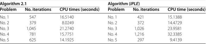
Example . The same as Example ., we only change the bifunction which has the form

f(x,y) =Px+Qy+q,y–x+d,arctan(x–y),

wherearctan(x–y) = (arctan(x–y), . . . ,arctan(x–y))T, the components ofdare chosen

Table 1 Example 4.1: Iterations of Algorithm 2.1 withr(xk) ≤0.0001

Iteration (k) xk

1 xk2 xk3 xk4 xk5

0 1 3 1 1 1

10 4.3842 0.0001 3.4633 1.7683 1.3842 20 4.4657 0.0013 3.1371 1.9315 1.4657 50 4.4901 0.0017 3.0404 1.9796 1.4898 100 4.4976 0.0082 3.0117 1.9938 1.4969 150 4.5001 0.0099 3.0031 1.9979 1.4990 180 4.5012 0.0107 3.0005 1.9989 1.4995 200 4.5106 0.0142 2.9716 2.0071 1.4965 250 4.5309 0.0412 2.9176 2.0206 1.4897 300 4.5370 0.0494 2.9013 2.0247 1.4877 350 4.5389 0.0519 2.8963 2.0259 1.4870 355 4.5395 0.0526 2.8948 2.0263 1.4868 358 4.5396 0.0528 2.8943 2.0264 1.4868 360 4.5397 0.0529 2.8942 2.0264 1.4868 361 4.5397 0.0529 2.8942 2.0265 1.4868

Table 2 Example 4.2: The tolerancer(xk) ≤0.19

Algorithm 2.1 Algorithm (IPLE)

Problem No. iterations CPU times (seconds) Problem No. iterations CPU time (seconds)

No. 1 547 16.5140 No. 1 421 15.1388

No. 2 379 8.0249 No. 2 372 14.4729

No. 3 1,045 21.2740 No. 3 1,026 23.9581

No. 4 781 15.7751 No. 4 1,216 32.3385

No. 5 625 14.1925 No. 5 297 9.4139

Then the bifunctionfsatisfies convergent assumptions of Theorem . in this paper and Theorem . in []. We choose the parameters in Algorithm .: ¯A–_{= ,β= ,σ= .,}

γ = .,μ= .. In the algorithm (shortly (IPLE)) proposed by Nguyen et al.[], the parameters are chosen as follows:θ= .,τ= .,α= .,μ= ,ck= . +_k_+for allk≥.

We compare Algorithm . with (IPLE). The iteration numbers and the computational time for  problems are given in Table .

The computations are performed by Matlab Ra running on a PC Desktop Intel(R) Core(TM)i @. GHz . GHz  Gb RAM.

5 Conclusion

Competing interests

The authors declare that they have no competing interests.

Authors’ contributions

The main idea of this paper is proposed by PNA. PNA and PMT prepared the manuscript initially and performed all the steps of proof in this research. All authors read and approved the final manuscript.

Author details

1_{Department of Scientific Fundamentals, Posts and Telecommunications Institute of Technology, Hanoi, Vietnam.} 2_{Academy of Military Science and Technology, Hanoi, Vietnam.}

Acknowledgements

We are very grateful to the anonymous referees for their really helpful and constructive comments in improving the paper. The work was supported by National Foundation for Science and Technology Development of Vietnam (NAFOSTED), code 101.02-2011.07.

Received: 10 July 2012 Accepted: 10 March 2013 Published: 5 April 2013 References

1. Blum, E, Oettli, W: From optimization and variational inequality to equilibrium problems. Math. Stud.63, 127-149 (1994)

2. Bigi, G, Castellani, M, Pappalardo, M: A new solution method for equilibrium problems. Optim. Methods Softw.24, 895-911 (2009)

3. Daniele, P, Giannessi, F, Maugeri, A: Equilibrium Problems and Variational Models. Kluwer Academic, Dordrecht (2003) 4. Konnov, IV: Combined Relaxation Methods for Variational Inequalities. Springer, Berlin (2000)

5. Moudafi, A: Proximal point algorithm extended to equilibrium problem. J. Nat. Geom.15, 91-100 (1999)

6. Anh, PN: Strong convergence theorems for nonexpansive mappings and Ky Fan inequalities. J. Optim. Theory Appl. (2012). doi:10.1007/s10957-012-0005-x

7. Anh, PN: A hybrid extragradient method extended to fixed point problems and equilibrium problems. Optimization (2012). doi:10.1080/02331934.2011.607497

8. Anh, PN, Kim, JK: Outer approximation algorithms for pseudomonotone equilibrium problems. Comput. Math. Appl. 61, 2588-2595 (2011)

9. Anh, PN, Muu, LD, Nguyen, VH, Strodiot, JJ: Using the Banach contraction principle to implement the proximal point method for multivalued monotone variational inequalities. J. Optim. Theory Appl.124, 285-306 (2005)

10. Iusem, AN, Sosa, W: On the proximal point method for equilibrium problems in Hilbert spaces. Optimization59, 1259-1274 (2010)

11. Zeng, LC, Yao, JC: Modified combined relaxation method for general monotone equilibrium problems in Hilbert spaces. J. Optim. Theory Appl.131, 469-483 (2006)

12. Heusinger, A, Kanzow, C: Relaxation methods for generalized Nash equilibrium problems with inexact line search. J. Optim. Theory Appl.143, 159-183 (2009)

13. Konnov, IV: Combined relaxation methods for monotone equilibrium problems. J. Optim. Theory Appl.111, 327-340 (2001)

14. Quoc, TD, Anh, PN, Muu, LD: Dual extragradient algorithms to equilibrium problems. J. Glob. Optim.52, 139-159 (2012)

15. Mastroeni, G: On auxiliary principle for equilibrium problems. In: Daniele, P, Giannessi, F, Maugeri, A (eds.) Equilibrium Problems and Variational Models. Nonconvex Optimization and Its Applications, vol. 68, pp. 289-298. Kluwer Academic, Dordrecht (2003)

16. Korpelevich, GM: The extragradient method for finding saddle points and other problems. Matecon12, 747-756 (1976)

17. Tran, DQ, Dung, ML, Nguyen, VH: Extragradient algorithms extended to equilibrium problems. Optimization57, 749-776 (2008)

18. Anh, PN: A logarithmic quadratic regularization method for solving pseudomonotone equilibrium problems. Acta Math. Vietnam.34, 183-200 (2009)

19. Bnouhachem, A: An LQP method for pseudomonotone variational inequalities. J. Glob. Optim.36, 351-356 (2006) 20. Forsgren, A, Gill, PE, Wright, MH: Interior methods for nonlinear optimization. SIAM Rev.44, 525-597 (2002) 21. Nguyen, TTV, Strodiot, JJ, Nguyen, VH: The interior proximal extragradient method for solving equilibrium problems.

J. Glob. Optim.44, 175-192 (2009)

22. Anh, PN: An LQP regularization method for equilibrium problems on polyhedral. Vietnam J. Math.36, 209-228 (2008) 23. Auslender, A, Teboulle, M, Bentiba, S: A logarithmic-quadratic proximal method for variational inequalities. Comput.

Optim. Appl.12, 31-40 (1999)

24. Auslender, A, Teboulle, M, Bentiba, S: Iterior proximal and multiplier methods based on second order homogeneous kernels. Math. Oper. Res.24, 646-668 (1999)

25. Bigi, G, Passacantando, M: Gap functions and penalization for solving equilibrium problems with nonlinear constraints. Comput. Optim. Appl.53, 323-346 (2012)

26. Marcotte, P: Algorithms for the network oligopoly problem. J. Oper. Res. Soc.38, 1051-1065 (1987)

27. Mordukhovich, BS, Outrata, JV, Cervinka, M: Equilibrium problems with complementarity constraints: case study with applications to oligopolistic markets. Optimization56, 479-494 (2007)

28. Murphy, FH, Sherali, HD, Soyster, AL: A mathematical programming approach for determining oligopolistic market equilibrium. Math. Program.24, 92-106 (1982)

doi:10.1186/1029-242X-2013-156

Cite this article as:Anh et al.:An interior approximal method for solving pseudomonotone equilibrium problems.