Synthesis of the Control of the Temperature Maintaining Process in a Heat Supply Problem

2018 IX International Conference on Optimization and Applications (OPTIMA 2018) ISBN: 978-1-60595-587-2

Synthesis of the Control of the Temperature Maintaining Process in a

Heat Supply Problem

Kamil AIDA-ZADE

_{and Vagif ABDULLAYEV}

Baku State University, st. Z. Xalilov 23, AZ1141 Baku, Azerbaijan

Institute of Control Systems of ANAS, st. B. Vahabzade 9, AZ1141 Baku, Azerbaijan Azerbaijan State Oil and Industry University, Azadlig ave. 20, AZ1010 Baku, Azerbaijan

Corresponding author

Keywords: Optimal control, Feedback, Loaded differential equation.

Abstract. _{We consider a problem of controlling a heating appliance used for heating a heat-}

transfer agent, which delivers heat into a closed system. To control the process, we use feedback, under which information on the process state is continuously or discretely received from individ- ual points of the appliance with installed temperature sensors. The mathematical model of the controlled process is described in both cases by a pointwise loaded first-order hyperbolic equation. We have obtained formulas for the gradient of the functional of the problem. These formulas allow us to use numerical first-order optimization methods for solving the problems. Numerical experiments have been carried out by the example of solving several test problems.

Introduction and Related Work

In the work, we propose an approach to the construction of a feedback control system for objects with distributed parameters. A heat supply system is chosen as the ob ject, into which enters fluid heated in the heat exchanger placed inside the steam jacket [21]. At some points of the heat exchanger, temperature sensors are installed. Depending on the readout of these sensors appropriate amount of heat is supplied to the heat exchanger. The heat exchange process in the heat exchanger is described by a hyperbolic equation. In the boundary conditions, there is a delayed time argument due to the time necessary for the hot fluid to flow through the heat supply system.

We note that a lot of work has been devoted to optimal feedback control problems for objects described by ordinary differential equations, in particular, by linear equations (see [15, 13, 20, 22, 7]). Feedback control problems for objects described by partial differential equations have been studied significantly less (see [21, 8, 9, 4]). Firstly, this is due to the complexity of the practical implementation of telemechanical control systems for objects distributed in space and time (see [17]). This is caused by the impossibility of continual or even discrete in time operative retrieval of information on the state of the entire object (at all its points). Secondly, there are problems with mathematical and computational nature that involve, in particular, initial- and boundary-value problems with respect to partial differential equations, requiring a long-term solution, which often does not allow constructing control systems for objects with distributed parameters in real-time mode.

1 2

3

The approach to the synthesis of the optimal control of the heat supply process proposed in the work uses information on the process state at a finite number of measurement points and moreover, the locations of the measurement points themselves are optimized. We have obtained formulas for the gradient of the target functional with respect to the optimizable feedback control parameters. These formulas can be used to solve the problem numerically using first-order optimization meth-ods, as well as to formulate the necessary optimality conditions in various forms – analogs of the Pontryagin maximum principle.

Problem Statement

The process of heating a heat-carrying agent in the furnace of the heated apparatus (heat exchanger) of the heating system can be described by the transport equation (see [21, 23]):

∂u(x, t)

∂t +a

∂u(x, t)

∂x =α[ϑ(t)−u(x, t)], (x, t)∈Ω = (0, l)×(0, T], (1)

where u = u(x, t) - is the temperature of the heat-carrying agent at the point x of the heat exchanger at the point of time t; l -the length of the heating tube, in which the heat-carrying agent is heated; a the velocity of the heat-carrying agent in the heat supply system, the value of which is constant for all points of the heat supply system, i.e. the motion is assumed to be steady (stationary); α the given value of the heat transfer coefficient between the furnace and the heat-carrying agent in the heating apparatus; ϑ(t) the temperature inside the furnace, by means of which the process of heating the heat-carrying agent is controlled, satisfying the technological limit:

ϑ≤ϑ(t)≤ϑ.¯ (2)

Let L be the linear length of the whole heat supply system, and L far exceeds l, i.e.L >> l. Then the heat-carrying agent heated in the furnace needs timeTd_{=L/a in order to return to the} beginning of the furnace, i.e.

u(0, t) = (1−γ)u(l, t−Td), t >0, (3)

γ is the constant value that determines the heat waste during the motion in the heating system, which, in essence, depends considerably on the temperature of the external environment. On the basis of practical considerations, we have the obvious condition:

0≤γ ≤1. (4)

Denote by Γ the set of all possible values ofγ, determining the amount of heat waste, satisfying (3), (4). It is assumed that a density functionρΓ(γ) on this set is given satisfying the condition:

ρΓ(γ)∈[0,1], γ ∈Γ.

Let the initial condition be given as:

u(x, t) = const, x∈[0, l], −Td< t <0. (5)

The problem of controlling the process of heating the heat-carrying agent consists in maintaining the furnace temperature at such a level that provides a certain temperaturez of the heat-carrying

agent at the exit of the furnace under all possible admissible values of the heat waste by the heat-carrying agent when it moves in the heat supply system, determined by the valuesγ ∈Γ .

Let sensors be installed at M arbitrary points ξi ∈[0, l], i= 1,2, ..., M, of the heating appara-tus, at which temperature measurements are taken continuously:

ui(t) = u(ξi, t), t∈[0, T], (6)

or at discrete points of time

uij =u(ξi, tj), tj ∈[0, T], j = 1,2, ..., m. (7)

To construct a heating control system with a continuous feedback, consider the following variant of the temperature control system:

ϑ(t) = 1

L

M X

i=1

λik˜i[u(ξi, t)−zi], (8)

where ˜ki is the amplification coefficient; zi the effective temperature at the point ξi, at which we need to control the amount of deviation from this value; λi = const the weighting coefficient, determining the importance of taking a measurement at the point ξi, i= 1,2, ..., M,

λ ∈Λ = (

λ∈EL: 0≤λi ≤1, i= 1,2, ..., M, M X

i=11 λi = 1

)

.

We introduce complex parameters:

ki =

λi˜ki

L , i= 1, 2, ..., M.

In this case the formula for the temperature in the furnace (8) takes the form:

ϑ(t) =ϑ(t;y) = M X

i=1

ki[u(ξi, t)−zi]. (9)

Here y = (ξ, k, z)∗ ∈ R3M is the vector of parameters of the feedback that determines the current control value (furnace temperature) depending on the measured temperature values at the heat exchanger measurement points; ”*” is the transposition sign.

Substituting (8) into (1), we obtain:

∂u(x, t)

∂t +a

∂u(x, t)

∂x =α

" _M X

i=1

ki[u(ξi, t)−zi]−u(x, t) #

,

(x, t)∈Ω = (0, l)×(0, T]. (10)

The minimized criterion of the control quality is given by the following form:

J(y;γ) = Z

I(y;γ) =β1

T Z

0

[u(l, t;y, γ)−V]2dt+σy−y0

2

R3L, (12)

where V - the given desired temperature in output. y0 = (ξ0, k0, z0)∗ ∈ R3M and σ ≥ 0 are regularization parameters.

Thus, the feedback control problem is reduced to a parametric optimal control problem. The reduced problem is described by the loaded differential equation (10)(see [14, 18, 12, 1, 11]) with boundary conditions involving a delayed argument (3).

On the optimizable feedback control parameters y we can impose, taking the designation (8) into account, some constraints on the basis of technical and technological considerations:

0≤ξi ≤l, ki ≤ki ≤¯ki, zi ≤zi ≤z¯i, i= 1, 2, ..., M. (13)

Here k_i, k¯i, zi, z¯i, i= 1, 2, ..., M, are the given values.

Derivation of the Formulas for the Gradient of the Functional

For numerical solution to the obtained problem of parametric optimal control of a loaded system with distributed parameters, we propose to use first-order methods, for example, the gradient projection method (see [16, 24, 19]). To construct a minimizing sequence yν_{, ν = 0,1, ...,, an} iterative process is constructed:

yν+1 =P(13)[yν −µνgrad J(yν)] , ν= 0,1, ..., (14)

Here P(13)(y) - is the projection operator of a three-dimensional pointy = (ξ, k, z)∗ on the set

defined by the constraints (13);µν >0 the step in the direction of the projected anti-gradient. The initial approximationy0 _{can be arbitrary, satisfying, in particular, the conditions (13). Considering}

the simplicity of the structure of the admissible set of optimizable parameters defined by the constraints (13), the projection operator has a constructive character and is easy to implement.

To build the procedure (14), we obtain formulas for the components of the gradient of the functional (11), (12) with respect to the optimizable parameters:

grad J(y) =

∂J(ξ, k, z)

∂ξ ,

∂J(ξ, k, z)

∂k ,

∂J(ξ, k, z)

∂z

∗

.

For this, we use the well-known technology of obtaining formulas for an increment of the functional obtained at the expense of the increment of the optimizable arguments of the functional (see [24]). In this case, the linear part of the increment of the functional with respect to each of the arguments will be the desired component of the gradient of the functional with respect to the corresponding argument.

Before proceeding to obtain formulas for the gradient components of the functional, we note the following. Taking into account that the parameter γ ∈ Γ, determining the amount of heat waste, does not depend on the process of heating the heat-carrying agent in the heat exchanger, from (11),(12) it follows that:

grad J(y) =grad

Z

Γ

I(y;γ)ρΓ(γ)dγ =

Z

Γ

grad I(y;γ)ρΓ(y)dγdy. (15)

Therefore we obtain the formula grad I(y;γ) for any one arbitrarily given heat wasteγ ∈Γ. Letu(x, t;y, γ) be the solution to the loaded initial- and boundary-value problem (10), (3), (5) for an arbitrary chosen vector of the optimizable parameters y= (ξ, k, z)∗ and for a given value of the heat waste parameterγ ∈Γ. For brevity, where this does not cause ambiguity, the parameters

y, γ will be omitted from the solution u(x, t;y, γ).

Let the parametersy= (ξ, k, z)∗have obtained some admissible increments ∆y = (∆ξ,∆k,∆z)∗ , and ˜u(x, t) = ˜u(x, t; ˜y) =u(x, t) + ∆u(x, t) be the solution to the problem (10), (3),(5), that cor-responds to the incremented vector of arguments ˜y=y+ ∆y.

Substituting the function ˜u(x, t) into the conditions (10), (3),(5), we obtain the following initial-and boundary-value problem accurate within the terms of the first order of smallness with respect to the increment ∆u(x, t) of the phase variable:

∆ut(x, t) +a∆ux(x, t) =α

M X

i=1

[ki∆u(ξi, t) +kiux(ξi, t)∆ξi+

+ (u(ξi, t)−zi) ∆ki−ki∆zi]−α∆u(x, t), (x, t)∈Ω, (16)

∆u(x,0) = 0, x∈[0, l], (17)

∆u(0, t) =

0, t ≤Td_,

(1−γ)∆u(l, t−Td), t≥Td. (18)

In obtaining formula (16) we used the relation:

u(ξi+ ∆ξi, t) = u(ξi, t) +ux(ξi, t)∆ξi+o(|∆ξi|).

For the increment of the functional (12), it is not difficult to obtain directly the representation:

∆I(y;γ) =I(˜y;γ)−I(y;γ) = I(y+ ∆y;γ)−I(y;γ) =

= 2β1

T R

0

[u(l, t;y, γ)−V] ∆u(l, t)dt+ 2σ 3M P

i=1

(yi −yi0)∆yi .

3M X

i=1

(yi−yi0)∆yi =

3M X

i=1

(ξi−ξi0)∆ξi+ (ki−ki0)∆ki+ (zi−zi0)∆zi

.

Let ψ(x, t) = ψ(x, t;y, γ) be yet an arbitrary function continuous everywhere on Ω, except points x=ξi, i= 1,2, ..., M, differentiable with respect to x for x ∈(ξi, ξi+1), i= 0,1, ..., M, ξ0 =

the functionψ(x, t;y, γ). We multiply equation (16) byψ(x, t) and integrate it over a rectangle Ω. Taking into account the assumed assumptions and conditions (17), (18), we have:

T Z 0 l Z 0

ψ(x, t)∆ut(x, t)dxdt+a M X

i=0

ξi+1

Z

ξi

T Z

0

ψ(x, t)∆ux(x, t)dtdx−

−α T Z 0 l Z 0

ψ(x, t) M X

i=1

[ki∆u(ξi, t) +kiux(ξi, t)∆ξi+ (u(ξi, t)−zi) ∆ki−ki∆zi]dx dt+

+α T Z 0 l Z 0

ψ(x, t)∆u(x, t)dx dt = 0. (19)

Using integration by parts for the first and second terms of (19) separately, and taking (17)–(18) into account, we obtain:

T Z 0 l Z 0

ψ(x, t)∆ut(x, t)dxdt=

= l Z

0

ψ(x, T)∆u(x, T)dx−

T Z 0 l Z 0

ψt(x, t)∆u(x, t)dxdt, (20)

a

M X

i=0

ξi+1

Z

ξi

T Z

0

ψ(x, t)∆ux(x, t)dtdx=a T Z

0

[ψ(l, t)∆u(l, t)−ψ(0, t)∆u(0, t)]dt+

+a M X i=1 T Z 0

ψ(ξ−_i , t)−ψ(ξ+_i , t) ∆u(ξi, t)dt−a T Z 0 l Z 0

ψx(x, t)∆u(x, t)dxdt=

=a

T Z

0

ψ(l, t)∆u(l, t)dt−a(1−γ) T Z

Td

ψ(0, t)∆u(l, t−Td)dt+

+a M X i=1 T Z 0

ψ(ξ−_i , t)−ψ(ξ+_i , t) ∆u(ξi, t)dt−a T Z 0 l Z 0

ψx(x, t)∆u(x, t)dxdt=

=a

T Z

0

ψ(l, t)∆u(l, t)dt−a(1−γ) T−Td

Z

0

ψ(0, t+Td)∆u(l, t)dt+

+a M X i=1 T Z 0

ψ(ξ_i−, t)−ψ(ξ_i+, t) ∆u(ξi, t)dt−a T Z 0 l Z 0

ψx(x, t)∆u(x, t)dxdt. (21)

Here we have used the notation

ψ(ξ_i−, t) =ψ(ξi−0, t), ψ(ξi+, t) =ψ(ξi+ 0, t).

Taking (19)–(21) into account, we obtain for the increment of the functional:

∆I =β1

T Z

T−Td

[aψ(l, t) + 2(u(l, t)−V)] ∆u(l, t)dt+ l Z

0

ψ(x, T)∆u(x, T)dx+

+ T−Td

Z

0

aψ(l, t) +a(1−γ)ψ(0, t+Td) + 2(u(l, t)−V)

∆u(l, t)dt+

+ T Z

0

l Z

0

[−ψt(x, t)−aψx(x, t) +αψ(x, t)]∆u(x, t)dxdt+

+a

M X

i=1

T Z

0



ψ(ξ

−

i , t)−ψ(ξ

+

i , t)−

α aki

l Z

0

ψ(x, t)dx



 ∆u(ξi, t)dt−

−α

T Z

0

l Z

0

ψ(x, t) M X

i=1

[kiux(ξi, t)∆ξi+ (u(ξi, t)−zi) ∆ki−ki∆zi]dx dt+

+ 2σ

M X

i=1

(ξi−ξi0)∆ξi+ (ki−k0i)∆ki+ (zi−zi0)∆zi

. (22)

Since the function ψ(x, t) is arbitrary, we require that it be almost everywhere a solution of the following adjoint initial- and boundary-value problem:

ψt(x, t) +aψx(x, t) = αψ(x, t), (x, t)∈Ω, (23)

ψ(x, T) = 0, x∈[0, l], (24)

ψ(l, t) = −2

a(u(l, t)−V), t∈(T −T

d

, T], (25)

ψ(l, t) = −α

a(1−γ)ψ(0, t+T

d₎₋ 2

a(u(l, t)−V), t ∈(0, T −T

d_{], (26)}

and at the points ξi, i= 1,2, ..., M for t ∈[0, T], it satisfy the condition:

ψ(ξ_i−, t) =ψ(ξ_i+, t) + α

aki

l Z

0

Taking into account that the components of the gradient of the functional are determined by the linear part of the increment of the functional under the increments of the corresponding arguments, we obtain:

gradξiI =−αki

T Z 0   l Z 0

ψ(x, t)dx



ux(ξi, t)dt+ 2σ(ξi−ξi0), i= 1,2, ...., M, (28)

gradkiI =−α

T Z

0

(u(ξi, t)−zi) 

 l Z

0

ψ(x, t)dx



dt+ 2σ(ki−k0i), i= 1,2, ...., M, (29)

gradziI =αki

l Z

0

ψ(x, t)dx+ 2σ(zi−zi0), i= 1,2, ...., M. (30)

The adjoint problem (23)-(27) can also be represented in another equivalent form, without the jump conditions (27). To do this, using the property of the δ function, we reduce the third term in (19) to the form:

a T Z 0 l Z 0

ψ(x, t) M X

i=1

(ki∆u(ξi, t) +kiux(ξi, t)∆ξi+ (u(ξi, t)−zi)∆ki−ki∆zi)dxdt=

=a L X i=1 ki T Z 0 l Z 0 l Z 0

ψ(ζ, t)δ(ζ−ξi)∆u(ζ, t)dζdxdt+

+a T Z 0 l Z 0

ψ(x, t) M X

i=1

(kiux(ξi, t)∆ξi+ (u(ξi, t)−zi)∆ki−ki∆zi)dxdt.

Changing the order of integration with respect to ζ and x in the first triple integral and renaming again the integration variables with respect to ζ and x between each other, we obtain:

T Z 0 l Z 0 l Z 0

ψ(ζ, t)δ(ζ−ξi)∆u(ζ, t)dζdxdt=

= T Z 0 l Z 0   l Z 0

ψ(ζ, t)dζ



δ(x−ξi)∆u(x, t)dxdt. (31)

Taking (31) into account in (19), in which, after making a rearrangement of the terms, instead of (23), (26) we obtain the following form of the adjoint problem:

ψt(x, t) +aψx(x, t) =αψ(x, t)−α l Z

0

ψ(ζ, t)dζ

M X

i=1

kiδ(x−ξi), (x, t)∈Ω, (32)

while preserving the initial and boundary conditions (24)-(26), but without the jump conditions (27).

Thus, we can consider the following theorem to be proved.

Theorem 1. Theorem. The gradient of the functional in the problem (10),(3)-(5), (11)–(12) for the admissible control parameters y= (ξ, k, z)∗ is determined by the formulas:

gradξiJ(y) =

Z

Γ







−αki T Z

0



 l Z

0

ψ(x, t;y, γ)dx



ux(ξi, t;y, γ)dt+

+ 2σ(ξi−ξi0) ρΓ(γ)dγ, i= 1,2, ...., M, (33)

gradkiJ(y) =

Z

Γ







−α

T Z

0

(u(ξi, t;y, γ)−zi) 

 l Z

0

ψ(x, t;y, γ)dx



dt+

+ 2σ(ki−k0i) ρΓ(γ)dγ, i= 1,2, ...., M, (34)

gradziJ(y) =

Z

Γ







αki l Z

0

ψ(x, t;y, γ)dx+ 2σ(zi−zi0) 





ρΓ(γ)dγ, i= 1,2, ...., M . (35)

whereu(x, t;y, γ), ψ(x, t;y, γ) are the solutions to the direct and adjoint boundary-value problems (10),(3)-(5) and (23)–(27), respectively.

For a numerical solution to the direct and adjoint boundary-value problems (8)-(13) and (23)-(27), taking into account their specific features, which is necessary for each iteration of the pro-cedure (14) when solving the initial optimization problem, one can use the grid method or the method of straight lines, investigated in (see [5, 10, 2, 3, 6]).

Results of the Numerical Experiments

We present the results of solving the following model problem. The process is described by the boundary value problem (1)-(5). It is necessary to design an optimal heating control (regulation) system with feedback at two points of the heating apparatus, that is, to solve the considered problem (1)-(5), (10)-(22) and determine ξ1, ξ2 the points of location of two temperature sensors,

control parameters ki, zi, i= 1, 2 .

The problem was solved for the following data: l = 1; a = 1; α = 0,1; Td _{= 1. The upper} admissible values of the control coefficient ¯ϑ= 100, the lower one, ϑ = 10. V = 85 andβ1 = 0,1;

the density function ρΓ(γ) was taken in the calculations as uniformly distributed ρΓ(γ) = 1/5; γi = 0,1i, i= 2,3,4,5,6.

The numerical experiments were carried out for computations initial values of the optimized parameters. Table 1 shows these values and the corresponding values of the functional.

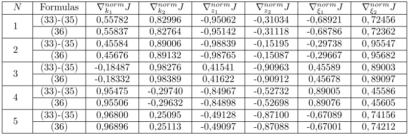
For each collection of the initial values of the optimized parameters, Table 2 presents the values of the components of the normalized gradients calculated by the proposed formulas (33)-(35) with the use of the difference approximation of the functional derivatives

∂J(y)

∂y ≈

J(y+εej)−J(y−εej)

whereyj is the j−th component of the optimizedN-dimensional vectoryrepresenting the totality of the optimized parameters ki, zi, ξi, i = 1, 2, ..., M, ej is the N-dimensional vector consisting of zeros save and except the j−th unit component. In the experiments, the value of ε was varied.

Table 1. Initial values of the optimized parametersk0₁,k₂0,z₁0,z₂0,ξ₁0,ξ0₂ and the corresponding values of the functional

N k0

1 k02 z10 z02 ξ10 ξ20 J0(y)

1 0,4 0,6 15 45 0,1 0,8 2657,210004

2 0,3 0,5 25 55 0,2 0,9 1557,150011

3 0,1 0,8 85 15 0,4 0,8 2557,310003

4 0,5 0,2 35 43 0,5 0,7 1165,150016

5 0,6 0,4 42 22 0,2 0,7 2005,190007

Table 2. Values of the components of the normalized gradients of functional calculated

N Formulas ∇norm

k1 J ∇

norm

k2 J ∇

norm

z1 J ∇

norm

z2 J ∇

norm

ξ1 J ∇

norm

ξ2 J

1 (33)-(35) 0,55782 0,82996 -0,95062 -0,31034 -0,68921 0,72456 (36) 0,55837 0,82764 -0,95142 -0,31118 -0,68786 0,72362

2 (33)-(35) 0,45584 0,89006 -0,98839 -0,15195 -0,29738 0,95547 (36) 0,45676 0,89132 -0,98765 -0,15087 -0,29667 0,95682

3 (33)-(35) -0,18487 0,98276 0,41541 -0,90963 0,45589 0,89003 (36) -0,18332 0,98389 0,41622 -0,90912 0,45678 0,89097

4 (33)-(35) 0,95475 -0,29740 -0,84967 -0,52732 0,89005 0,45586 (36) 0,95506 -0,29632 -0,84898 -0,52698 0,89076 0,45605

5 (33)-(35) 0,96800 0,25095 -0,49128 -0,87100 -0,67089 0,74156 (36) 0,96896 0,25113 -0,49097 -0,87088 -0,67001 0,74212

Table 3. Values of the optimized parameters and the corresponding values of the functional obtained at the sixth iteration

N k(6)₁ k(6)₂ z₁(6) z₂(6) ξ(6)₁ ξ₂(6) J(6)(y)

1 0,1956 0,2959 63,9945 60,9949 0,2994 0,5994 0,000122 2 0,1977 0,3003 63,9978 60,9954 0,3000 0,6000 0,000059 3 0,1962 0,2988 63,9951 60,9948 0,2971 0,5971 0,000121 4 0,1978 0,2941 63,9991 60,9975 0,3000 0,6000 0,000075 5 0,1991 0,2961 63,9964 60,9973 0,3000 0,6000 0,000065

Table 3 compiles the values of the parameterski, zi, ξi, i= 1, 2, ..., M obtained at the seventh iteration of the method of projection of the conjugate gradient from the initial points given in Table 1.

Conclusion

Automatic feedback control systems for technical objects and technological processes with dis-tributed parameters are widely used owing to the significantly increased capabilities of measuring

and computing facilities. In the paper, we investigated the problem of controlling a heating appa-ratus for heating a heat-carrying agent, which ensures the supply of heat to a closed heat supply system. The specificity of the investigated problem, described by the first-order hyperbolic equa-tion, lies in the fact that in its boundary conditions a delayed in time argument takes part. The mathematical model of the controlled process is reduced to a pointwise-loaded hyperbolic equation, and the problem under consideration is reduced to the parametric optimal control problem. In or-der to use first-oror-der optimization methods for the numerical solution to the problem of optimizing the locations of sensors and the parameters of feedback control actions, we obtained formulas for the corresponding gradient components of the target functional of the problem. The formulation of the problem and the approach to obtaining computational formulas for its numerical solution proposed in this paper can be extended to cases of feedback control by many other processes described by other types of partial differential equations.

References

[1] V.M. Abdullaev and K.R. Aida-zade. Numerical Solution of Optimal Control Problems for Loaded Lumped Systems, Comput. Math. Math. Phys. 46, 9 (2006) 1487–1502.

[2] V.M. Abdullaev and K.R. Aida-zade. On the Numerical Solution of Loaded Systems of Ordi-nary Differential Equations, Comput. Math. Math. Phys. 44, 9 (2004) 1585–1595.

[3] V.M. Abdullaev and K.R. Aida-zade. Numerical Method of Solution to Loaded Nonlocal Boundary Value Problems for Ordinary Differential Equations, Comput. Math. Math. Phys.

54,7 (2014) 1096–1109.

[4] V.M. Abdullayev and K.R. Aida-zade. Numerical Solution of the Problem of Determining the Number and Locations of State Observation Points in Feedback Control of a Heating Process, Comput. Math. Math. Phys.58,1 (2018) 78–89.

[5] V.M. Abdullayev and K.R. Aida-zade. Optimization of Loading Places and Load Response Functions for Stationary Systems, Comput. Math. Math. Phys. 57, 4 (2017) 634–644.

[6] V.M. Abdullayev and K.R. Aida-zade. Finite-difference Methods for Solving Loaded Parabolic Equations, Comput. Math. Math. Phys. 56, 1 (2016) 93–105.

[7] K.R. Aida-zade. An Approach to the Design of Lumped Controls in the Distributed Systems, Avtomat. Vychisl. Tekhn.3 (2005) 16–22.

[8] K.R. Aida-zade and V.M. Abdullaev. On an Approach to Designing Control of the Distributed-Parameter Processes, Autom. Remote Control. 73, 9 (2012) 1443–1455.

[9] K.R. Aida-zade and V.M. Abdullaev. Optimizing placement of the control points at synthesis of the heating process control, Autom. Remote Control. 78, 9 (2017) 1585–1599.

[10] K.R. Aida-zade and V.M. Abdullaev. On the solution of boundary-value problems with non-separated multipoint and integral conditions, Differential Equations. 49, 9 (2013) 1114–1125. [11] K.R. Aida-zade and V.M. Abdullayev. Solution of a Class of the Inverse Problems for Sys-tem of Loaded Ordinary Differential Equations Ordinary Differential Equations with Integral Conditions, J. Inverse Ill-posed Probl. 24, 5 (2016) 543–558.

[12] A.A. Alikhanov, A.M. Berezgov, and M.Kh. Shkhanukov-Lafshiev. Boundary value Problems for Certain Classes of Loaded Differential Equations and Solving Them by Finite Difference Methods, Comput. Math. Math. Phys. 48, 9 (2008) 1581–1590.

[14] M.T. Dzhenaliev. Optimal Control of Linear Loaded Parabolic Equations, Differ. Equations

25, 4 (1989) 641–651.

[15] A.I. Egorov. Fundamentals of the Control Theory, Moscow: Fizmatlit, (2004).

[16] Yu. G. Evtushenko. Methods for Solving Optimization Problems and Their Applications in Optimization Systems, Moscow: Nauka, (1982).

[17] J.L. Lions. Controle optimal des syst‘emes gouvern’es par des ’equations aux deriv’ees par-tielles, Paris: Dunod Gauthier-Villars, (1968).

[18] A.M. Nakhushev. Loaded Equations and Their Application, Moscow: Nauka, (2012). [19] B.T. Polyak. Introduction to Optimization, New York: Optimization Software, (1987). [20] B.T. Polyak and P.S. Shcherbakov. Robust Stability and Control, Moscow: Nauka, (2002). [21] W.H. Ray. Advanced Process Control, New York: McGraw-Hill, (1981).

[22] I.V. Sergienko and V.S. Deineka. Optimal Control of Distributed Systems with Conjugation Conditions, New York: Kluwer, (2005).

[23] A.N. Tikhonov and A.A. Samarskii. Equations of Mathematical Physics, Moscow: Nauka, (1966).

[24] F.P. Vasil’ev. Methods of Optimization, Moscow: Faktorial Press, (2002).