Gamma distribution approach in chance constrained stochastic programming model

R E S E A R C H

Open Access

Gamma distribution approach in

chance-constrained stochastic programming model

Kumru D Atalay

and Aysen Apaydin

* Correspondence: [email protected]

1_{Department of Medical Education,}

Faculty of Medicine, 06490, Bahçelievler, Ankara, Turkey Full list of author information is available at the end of the article

Abstract

In this article, a method is developed to transform the chance-constrained programming problem into a deterministic problem. We have considered a chance-constrained programming problem under the assumption that the random variablesaijare

independent with Gamma distributions. This new method uses estimation of the distance between distribution of sum of these independent random variables having Gamma distribution and normal distribution, probabilistic constraint obtained via Essen inequality has been made deterministic using the approach suggested by Polya. The model studied on in practice stage has been solved under the assumption of both Gamma and normal distributions and the obtained results have been compared.

Keywords:chance-constrained programming, Essen inequality, Gamma distribution

1. Introduction

A chance-constrained stochastic programming (CCSP) models is one of the major approaches for dealing with random parameters in the optimization problems. Charnes and Cooper [1] have first modelled CCSP. Here, they have developed a new conceptual and analytic method which contains temporary planning of optimal stochastic decision rules under uncertainty. Symonds [2] has presented deterministic solutions for the class of chance-constraint programming problem. Kolbin [3] has examined the risk and indefiniteness in planning and managing problems and presented chance-con-straint programming models. Stancu-Minasian [4] has suggested a minimum-risk approach to multi-objective stochastic linear programming problems. Hulsurkar et al. [5] have studied on a practice of fuzzy programming approach of multi-objective sto-chastic linear programming problems. They have used fuzzy programming approach for finding a solution after changing the suggested stochastic programming problem into a linear or a nonlinear deterministic problem. Liu and Iwamura [6] have studied on chance-constraint programming with fuzzy parameters. Chance-constraint program-ming in stochastic is expanded to fuzzy concept by their studies. They have presented certain equations with chance constraint in some fuzzy concept identical to stochastic programming. Furthermore, they have suggested a fuzzy simulation method for chance constraints for which it is usually difficult to be changed into certain equations. Finally, these fuzzy simulations which became basis for genetic algorithm have been suggested for solving problems of this type and discussing numeric examples. Mohammed [7] has studied on chance-constraint fuzzy goal programming containing right-hand side

values with uniform random variable coefficients. He presented the main idea related with the stochastic goal programming and chance-constraint linear goal programming. Kampas and White [8] have suggested the programming based on probability for the control of nitrate pollution in their studies and compared this with the approaches of various probabilistic constraints. Yang and Wen [9] presented a chance-constrained programming model for transmission system planning in the competitive electricity market environment. Huang [10] provided two types of credibility-based chance-con-strained models for portfolio selection with fuzzy returns. Ağpak and Gökçen [11] developed new mathematical models for stochastic traditional and U-type assembly lines with a chance-constrained 0-1 integer programming technique. Henrion and Strugarek [12] investigated the convexity of chance constraints with independent ran-dom variables. Parpas and Rüstem [13] proposed a stochastic algorithm for the global optimization of chance-constrained problems. They assumed that the probability mea-sure used to evaluate the constraints is known only through its moments. Xu et al. [14] developed a robust hybrid stochastic chance-constraint programming model for supporting municipal solid waste management under uncertainty. Abdelaziz and Masri [15] proposed a chance-constrained approach and a compromise programming approach to transform the multi-objective stochastic linear program with partial linear information on the probability distribution into its equivalent uni-objective problem. Goyal and Ravi [16] presented a polynomial time approximation scheme for the chance-constrained knapsack problem when item sizes are normally distributed and independent of other items.

The classical linear programming problem, which is a specific class of mathematical programming problem, is formulated as follows

maxz(x) =

n

j=1

cjxj

n

j=1

aijxj≤bi i= 1, ...,m

xj≥0 j= 1, ...,n

where all coefficients (technologic coefficientsaij, right-hand side valuesbiand

objec-tive function coefficientscj(j= 1,...,n i= 1,...,m)) are deterministic. However, when at

least one coefficient is a random variable, the problem becomes a stochastic program-ming problem.

In this article, we have assumed that theaij, (i= 1,...,m, j= 1,...n) which are the

ele-ments of, m×ntype technologic matrixA, are random variables having Gamma dis-tribution. In case that these coefficients having Gamma distribution are independent, the estimation of the distance between the distribution of sum of them and normal distribution has been obtained. Essen inequality has been used for these and determi-nistic equality of chance constraints has been found. The model with random variable coefficients has been solved via the suggested method and it has been implemented on a numeric example. The model has been examined again for the case to have coeffi-cients with normal distribution. It has been observed that the case aijcoefficients have

Gamma distribution or normal distribution has given similar results for large values of

2. Chance-constrained stochastic programming

Stochastic programming deals with the case that input data (prices, right hand side vector, technologic coefficients) are random variables. As parameters are random vari-ables, a probability distribution should be determined. Two frequently used approaches for transforming stochastic programming problem into a deterministic programming problem are chance constraint programming and two-staged programming.

“Chance-constrained programming”which is a stochastic programming method con-tains fixing the certain appropriate levels for random constraints. Therefore, it is generally used for modelling technical or economic systems. The practices include economic plan-ning, input control, structural design, inventory, air and water quality management pro-blems. In chance constraints, each constraint can be realized with a certain probability.

Stochastic linear programming problem with chance constraints is defined as follows

max(min)z(x)=

n

j=1

cjxj

P ⎡

⎣n

j=1

aijxj≤bi ⎤

⎦_≥1−ui

xj≥0, j= 1, ...,n

ui∈(0, 1), i= 1, ...,m

(2:1)

wherecj,aijandbiare random variables andui’s are chosen probabilities.kth chance

constraint given in model (2.1) is obtained as

P ⎡

⎣n

j=1

akjxj≤bk ⎤

⎦_≥1−uk (2:2)

with lower bound (1 -uk). Where it is assumed thatxj decision variables are

deter-ministic.cj,akjandbkare random variables with known variances and means [17,18].

If bkis the random variable in the model, and its distribution function isFbthen the

deterministic equivalent of chance constraint can be calculated as Pakjxj≤bk

≥uk⇔ P

bk≥akjxj

≥uk

⇔1−Fb akjxj

≥uk

⇔akjxj≤F−_b1(1−uk)

(2:3)

Assume that akj is a random variable having normal distribution with the meanE

(akj) and the varianceVar(akj). Furthermore, covariance between the random variables akjandaklis zero. Then, random variabledkis defined as follows

dk= n

j=1

akjxj

whereak1,..., akn’s are random variables with normal distribution and x1,...,xn’s are

unknowns, chance constraint given with inequality (2.2) is defined as follows

φ

bk−E(dk)

Var(dk)

≥φ Kuk

where Kuk denotes the value of standard normal variable and φ Kuk

= 1−uk.

Therefore, deterministic equivalent of inequality (2.4) is stated as E(dk)+Kuk

Var(dk)≤bk

Solution methods for models constituted by dual and triple combinations of cj,akj

andbkcoefficients and also for the case thatcj’s are random variable are different. In

this article, these are not mentioned [5,19-21]. 3. Gamma distribution approach for CCSP

Let, X1, X2,...,Xnbe independent random variables with a distribution functionFn(x).

LetF(x) be a standard normal distribution function. Then, supremum of absolute dis-tance between Fn(x) and F(x) can be found. The theorem related to this, which is

known as Essen Inequality, is as follows.

Theorem 3.1Let X1,X2,...,Xnbe independent random variables with given

EXj= 0and E|Xj|3<∞j= 1, ...,n

where if it is as follows

σ2

j =EX2j, ...,Bn= n

j=1

σ2

j , ...,Fn(x) =P ⎡ ⎣B−n1/2

n

j=1 Xj<x

⎤

⎦, ...,Ln=B−−n 3/2 n

j=1 E|Xj|3

then

sup

x |

Fn(x)−(x)|≤SLn ₍₃:₁₎

is defined. Here, S is an absolute positive constant[22].

Proof to Theorem 3.1 can be found in [[22], pp. 109-111]. In case of equality, as a result of Essen inequality we can give the following equation, for large values ofn

P

⎡ ⎣B−n1/2

⎛ ⎝n

j=1 Xj−E

⎛ ⎝n

j=1 Xj

⎞ ⎠ ⎞ ⎠_<x

⎤ ⎦=φ (x)+

n

j=1

EXj−E Xj3e

−x2 2 1−x2

6√2πB 3 2

n

+o(n−21₎ (3:2)

Equation 3.2 is used for approximation to standard normal distribution [23].

After defining the Essen inequality given in Theorem 3.1, now we explain Gamma distribution approach for CCSP model. In linear programming, the constraints are con-structed as follows:

Ax≤b⇔

⎡ ⎢ ⎢ ⎢ ⎢ ⎢ ⎢ ⎢ ⎢ ⎢ ⎣

a11a12...a1n

..

. ... . .. ...

ak1ak2...akn

..

. ... . .. ...

am1am2...amn ⎤ ⎥ ⎥ ⎥ ⎥ ⎥ ⎥ ⎥ ⎥ ⎥ ⎦

⎡ ⎢ ⎢ ⎢ ⎢ ⎢ ⎢ ⎢ ⎢ ⎢ ⎣

x1 .. .

xk

.. .

xn ⎤ ⎥ ⎥ ⎥ ⎥ ⎥ ⎥ ⎥ ⎥ ⎥ ⎦

≤

⎡ ⎢ ⎢ ⎢ ⎢ ⎢ ⎢ ⎢ ⎢ ⎢ ⎣

b1 .. .

bk

.. .

bm ⎤ ⎥ ⎥ ⎥ ⎥ ⎥ ⎥ ⎥ ⎥ ⎥ ⎦

(3:3)

Here, the matrixAindicates a coefficients matrix. Letdk =ak’x k= 1,...,mthenkth

dk≤bk⇔[ak1,ak2, ...,akn] ⎡ ⎢ ⎢ ⎢ ⎢ ⎢ ⎢ ⎣

x1 .

xk

.

xn ⎤ ⎥ ⎥ ⎥ ⎥ ⎥ ⎥ ⎦

≤ bk (3:4)

If akj’s which arekth row of coefficients matrixAare independent gamma random

variables, chance constraints given in model (2.1) are as follows

P(dk≤bk)≥1−uk, k= 1, 2, ...,m (3:5)

Assume that each random variable akjhas Gamma distribution with (akj, bkj)

para-meters in (3.4). For the purpose of using Essen inequality given in Theorem 3.1, the random variable rj =akjxj -E(akjxj),j = 1,...,nis taken into account. Expected value

and variance of each random variable akjas follows:

E(akj) =αkjβkj Var(akj) =αkjβkj2

Therefore, the expected value of random variablerjwill be as follows:

E(rj) =E(akjxj−E(akjxj)) =xj

αkjβkj−αkjβkj

= 0

and its variance will be as follows: Var(rj) =E(dj)2−

E(dj) 2

=x2_jVar(akj) =x2jαkjβkj2

Absolute third moment of random variabledjis found in the following equality

E|rj|3=E|akjxj−E(akjxj)|3=x3jE|akj−αkjβkj|3 (3:6)

The expected value in equality (3.6) can be written as follows:

Eakj−αkjβkj

3

=

∞

0

akj−αkjβkj

3 f(akj)dakj

=

αkjβkj

0

akj−αkjβkj3f(akj)dakj+ ∞

αkjβkj

akj−αkjβkj3f(akj)dakj

= Ikj+ IIkj (3:7)

Then, Ikjis rewritten as follows

Ikj= αkjβkj

0

− akj−αkjβkj 3

f(akj)dakj

=− 1

(αkj)β_kjαkj αkjβkj

0

a3_kj−3a2_kjαkjβkj+ 3akjα2kjβkj2−α3kjβkj3

aαkj−1

kj e −akj/_βkj

dakj

If it is taken as, − 1

(αkj)β_kjαkj

= _{in integral thenIkjcan be written as follows}

Ikj=

αkjβkj

0

aα_kjkj+2e−akj/βkj_da

kj− 3αkjβkj

αkjβkj

0

aα_kjkj+1e−akj/βkj_da

kj+

3α2kjβkj2

αkjβkj

0 aαkj

kje

−akj/βkj_da

kj

− α3

kjβ3kj

αkjβkj

0 aαkj−1

kj e

−akj/_βkjda

kj

= _ω1+ 3αkjβkj

ω2+

3_α2

kjβkj2

ω3+

α3

kjβkj3

Here, by making variable change _βakj

kj

=tkj,

ω1=βαkj

+3 kj

αkj

0

tαkj+2

kj e−tkjdtkj

is obtained. Incomplete gamma function is defined as follows I(a,x) = γ(a,x)

(a)

here

γ(a,x) =

x

0

ta−1e−tdt

Therefore, ω1can be rearranged as follows:

ω1=βαkj

+3

kj (αkj+ 3)I(αkj+ 3,αkj)

Similarly, it can be written as follows

ω2=βαkj

+2

kj (αkj+ 2)I(αkj+ 2,αkj)

ω3=βαkj

+1

kj (αkj+ 1)I(αkj+ 1,αkj)

ω4=β_kjαkj(αkj)I(αkj,αkj)

The second part of the integral can be written as follows

IIkj= ∞

αkjβkj

akj−αkjβkj 3

f(akj)dakj

= 1

(αkj)βkjαkj ∞

αkjβkj

a3_kj−3a2_kjαkjβkj+ 3akjα2kjβ 2 kj−α

3 kjβ

3 kj

aα_kjkj−1e−akj/βkj_da

kj

If it is taken as 1

(αkj)β_kjαkj

=− _{in integral then IIkjcan be written as follows}

IIkj=−

∞

αkjβkj aαkj+2

kj e

−a_kj/β

kj_da

kj+ 3αkjβkj

∞

αkjβkj aαkj+1

kj e

−a_kj/β

kj_da

kj−

3α2

kjβkj2

∞

αkjβkj aαkj

kje

−a_kj/β

kj_da

kj

+ α3

kjβkj3

∞

αkjβkj aαkj−1

kj e

−akj/_βkjda

kj

=− ξ1+ 3αkjβkj

ξ2−

3α2

kjβkj2

ξ3+

α3

kjβkj3

ξ4

where

ξ1=

∞

0

aαkj+2

kj e −akj_/β

kj_da

kj− αkjβkj

0

aαkj+2

kj e −akj_/β

kj_da

kj

=βαkj+3

kj (αkj+ 3)

1−I(αkj+ 3,αkj)

In the same way it will be

ξ2=βαkj

+2

kj (αkj+ 2)

1−I(αkj+ 2,αkj)

ξ3=β_kjαkj+1(αkj+ 1)

1−I(αkj+ 1,αkj)

ξ4=β_kjαkj(αkj)

1−I(αkj,αkj)

.

Therefore, for any finite akjandbkj, it can easily be seen thatEdj= 0 andE|dj|3<∞.

Therefore, the conditions in Theorem 3.1 are satisfied, then σj2 andBnis obtained as

σ2

j =Erj2=x2jαkjβkj2

Bn= n

j=1

σ2

j = n

j=1

x2_jαkjβkj2

The third absolute moment of random variable, rj, in terms of integrals Ikj and IIkjis

written as follows

E|rj|3=x3j Ikj+ IIkj

Then, Lnis obtained as follows

Ln=B −_3/2 n

n

j=1

Erj3 = n j=1

x3_j Ikj+IIkj

n j=1

x2 jαkjβkj2

_3/2 (3:8)

Even if Lndefined in Theorem 3.1 is maximum it can be a useful upper bound for

left side of (3.1). Following lemma is related to this situation.

Lemma 3.1Maximum value of Lnin Equation 3.8 is given by

maxLn=

nL∗

nx∗α∗(β∗)23/2

= nL

∗

n3/2(x∗α∗)3/2(β∗)3 (3:9)

ProofMaximum value ofLngiven in Equation 3.8 is obtained by maximizing

nomi-nator while minimizing the denominomi-nator, i.e.

max

j n

j=1

x3_j Ikj+ IIkj

and

min

j ⎡

⎣n

j=1

x2_jαkjβkj2 ⎤ ⎦ 3/2

Therefore,

max

j

x3_j Ikj+IIkj=L∗

and

min

j |x 2

equalities are defined. Then maximum value of Lngiven in Equation 3.8 is found as

Equation 3.9. This completes the proof of Lemma 3.1.

In Theorem 3.1, using Lngiven in (3.8), following inequality is obtained

sup

x |

Fn(x)−(x)|≤SLn

sup

x |

Fn(x)−(x)|≤S n j=1

x3_j Ikj+IIkj n j=1 x2 jαkjβkj2

_3/2 (3:10)

If the suggested constantS= 0.7975 [22] in inequality (3.10) and if the value max Ln

given with (3.9) is used following inequality is obtained

sup

x |

Fn(x)−(x)|≤0.7975

L∗ √

n(x∗α∗)3/2(β∗)3 (3:11)

Here, Fn(x) is Gamma distribution function,F(x) is that of standard normal

distribu-tion. Thus, fordk

dk− n j=1

xjE(akj)

n j=1

x2 jVar(akj)

=

dk− n j=1

xjαjβj

n j=1

x2 jαjβj2

is defined. Therefore, constraint (3.5) can be written as follows

P ⎡ ⎢ ⎢ ⎢ ⎢ ⎣ n j=1

akjxj− n j=1

xjαjβj

n j=1

x2 jαjβj2

≤ bk−

n j=1

xjαjβj

n j=1

x2 jαjβj2

⎤ ⎥ ⎥ ⎥ ⎥

⎦≥1−(uk+SLn)

Here, the following inequality is written

⎡ ⎢ ⎢ ⎢ ⎢ ⎣

bk− n j=1

xjαjβj

n j=1

x2_jαjβj2 ⎤ ⎥ ⎥ ⎥ ⎥

⎦≥1−(uk+SLn). (3:12)

There are decision variables xj (j = 1,..., n) in Ln which is on the left side of the

inequality (3.12). Since these decision variables are the results of the problem solved after model (2.1) is made deterministic, they are unknown here. Therefore,Ln is not a

numeric and it cannot be solved using F-1(1-(uk)+SLn). Therefore, using the approach

suggested [24] right side of inequality (3.12) can be written as follows

⎡ ⎢ ⎢ ⎢ ⎢ ⎣

bk− n j=1

xjαjβj

n j=1

x2 jαjβj2

⎤ ⎥ ⎥ ⎥ ⎥ ⎦= 1 2 ⎛ ⎜ ⎜ ⎜ ⎜ ⎜ ⎜ ⎝ 1 + ⎧ ⎪ ⎪ ⎪ ⎪ ⎨ ⎪ ⎪ ⎪ ⎪ ⎩

1−exp

⎛ ⎜ ⎜ ⎜ ⎜ ⎝− 2 π ⎡ ⎢ ⎢ ⎢ ⎢ ⎣

bk− n j=1

xjαjβj

n j=1

x2 jαjβj2

⎤ ⎥ ⎥ ⎥ ⎥ ⎦ 2⎞ ⎟ ⎟ ⎟ ⎟ ⎠ ⎫ ⎪ ⎪ ⎪ ⎪ ⎬ ⎪ ⎪ ⎪ ⎪ ⎭ 1/2⎞ ⎟ ⎟ ⎟ ⎟ ⎟ ⎟ ⎠

and deterministic constraint belonging to inequality (3.12) is then written as fallows 1 2 ⎛ ⎜ ⎜ ⎜ ⎜ ⎜ ⎜ ⎝ 1 + ⎧ ⎪ ⎪ ⎪ ⎪ ⎨ ⎪ ⎪ ⎪ ⎪ ⎩

1−exp

⎛ ⎜ ⎜ ⎜ ⎜ ⎝− 2 π ⎡ ⎢ ⎢ ⎢ ⎢ ⎣

bk− n

j=1 xjαjβj

n

j=1 x2

jαjβj2

⎤ ⎥ ⎥ ⎥ ⎥ ⎦ 2⎞ ⎟ ⎟ ⎟ ⎟ ⎠ ⎫ ⎪ ⎪ ⎪ ⎪ ⎬ ⎪ ⎪ ⎪ ⎪ ⎭ 1/2⎞ ⎟ ⎟ ⎟ ⎟ ⎟ ⎟ ⎠

≥1−

⎡ ⎢ ⎢ ⎢ ⎢ ⎢ ⎢ ⎣

uk+ 0.7975

⎛ ⎜ ⎜ ⎜ ⎜ ⎜ ⎜ ⎝ n j=1 x3

j Ikj+IIkj

n j=1 x2

jαkjβkj2

3/2 ⎞ ⎟ ⎟ ⎟ ⎟ ⎟ ⎟ ⎠ ⎤ ⎥ ⎥ ⎥ ⎥ ⎥ ⎥ ⎦

. (3:14)

Using Equation (3.2) we can construct the following inequality

1 2 ⎛ ⎜ ⎜ ⎜ ⎜ ⎜ ⎜ ⎝ 1 + ⎧ ⎪ ⎪ ⎪ ⎪ ⎨ ⎪ ⎪ ⎪ ⎪ ⎩

1−exp

⎛ ⎜ ⎜ ⎜ ⎜ ⎝− 2 π ⎡ ⎢ ⎢ ⎢ ⎢ ⎣

bk− n j=1 xjαkjβkj n j=1

x2_jαkjβ_kj2 ⎤ ⎥ ⎥ ⎥ ⎥ ⎦ 2⎞ ⎟ ⎟ ⎟ ⎟ ⎠ ⎫ ⎪ ⎪ ⎪ ⎪ ⎬ ⎪ ⎪ ⎪ ⎪ ⎭ 1/2⎞ ⎟ ⎟ ⎟ ⎟ ⎟ ⎟ ⎠

≥1−

⎡ ⎢ ⎢ ⎢ ⎢ ⎢ ⎢ ⎢ ⎢ ⎢ ⎢ ⎢ ⎢ ⎢ ⎢ ⎢ ⎢ ⎢ ⎢ ⎢ ⎢ ⎢ ⎢ ⎢ ⎢ ⎢ ⎢ ⎢ ⎢ ⎢ ⎣

uk+ n j=1

x3

j2αkjβkj3e

− ⎛ ⎜ ⎜ ⎜ ⎜ ⎝

bk− n j=1 xjαkjβkj n j=1

x2_jαkjβ_kj2 ⎞ ⎟ ⎟ ⎟ ⎟ ⎠ 2 2 ⎛ ⎜ ⎜ ⎜ ⎜ ⎝1−

⎛ ⎜ ⎜ ⎜ ⎜ ⎝

bk− n j=1 xjαkjβkj n j=1 x2

jαkjβkj2 ⎞ ⎟ ⎟ ⎟ ⎟ ⎠ 2⎞ ⎟ ⎟ ⎟ ⎟ ⎠

6√2π

# n j=1

x2

jαkjβkj2 $3 2 ⎤ ⎥ ⎥ ⎥ ⎥ ⎥ ⎥ ⎥ ⎥ ⎥ ⎥ ⎥ ⎥ ⎥ ⎥ ⎥ ⎥ ⎥ ⎥ ⎥ ⎥ ⎥ ⎥ ⎥ ⎥ ⎥ ⎥ ⎥ ⎥ ⎥ ⎦ (3.15)

4. Numerical experiments Consider the CCSP model as follows

maxz= 7x1+ 2x2+ 4x3

P[a11x1+a12x2+a13x3≤8]≥0.95

P5x1+x2+ 6x3≤b2

≥0.10

xj≥0 j= 1, 2, 3

(4:1)

Here, assume that akj j = 1,2,3 are independent random variables distributed as

Gamma distribution with the following parameters (akj,bkj)

α11= 4, β11= 1, α12= 2, β12= 2,α13= 3, β13= 2. (4:2)

b2is normal random variable with the following expected value and variance

E(b2)= 7, Var(b2)= 9

rj=akjxj−E akjxj

here, Var rj

=x2_j αkjβkj2

is found and fork= 1,Bnis obtained as follows

Bn= 4x21+ 8x22+ 12x23

Then, Lnis written as follows

Ln= 3 j=1

x3

j Ikj+ IIkj

4x2₁+ 8x2₂+ 12x2₃3/2

As a result of the solution of the integrals, Ikj (k= 1,j = 1,2,3) and IIkj (k= 1, j=

1,2,3) inLncan be obtained as

I11= 3.2824, II11= 11.2824

I12= 6.9766, II12= 38.9766

I13= 15.3291, II13= 63.3291

Then, Lnis found as

Ln=

14.5648x3

1+ 45.9532x32+ 78.6582x33

4x2₁+ 8x2₂+ 12x2₃3/2

.

Therefore, in the case where akj is a random variable with Gamma distribution,

deterministic equality of the first chance constraint in model (4.1), using inequality (3.14) is obtained as follows

1 2 ⎡ ⎢ ⎢ ⎢ ⎣1 +

⎧ ⎪ ⎨ ⎪ ⎩1−exp

⎛ ⎜ ⎝−2_π

⎡ ⎢

⎣8_%−(4x1+ 4x2+ 6x3) 4x2

1+ 8x22+ 12x23 ⎤ ⎥ ⎦ 2⎞

⎟ ⎠ ⎫ ⎪ ⎬ ⎪ ⎭

1/2⎤ ⎥ ⎥ ⎥ ⎦≥1−

⎡

⎣0.05 + 0.7975 ⎛ ⎝14.5648x3

1+ 45.9532x32+ 78.6582x33 4x2

1+ 8x22+ 12x23 3/2

⎞ ⎠ ⎤ ⎦ _(4:3)

Using inequality (3.15) we can write as:

0.5

⎛ ⎝1 +

&

1−exp

#

−0.6366(8−x4)

x5

2$'1/2⎞

⎠≥0.95−

⎡ ⎢ ⎢ ⎣(8x

3

1+ 32x32+ 48x33)e

−x6 2 (1−x6)

6(6.28)x

3 2 5

⎤ ⎥ ⎥ ⎦

x4−4x1−4x2−6x3= 0

x5−(4x21+ 8x22+ 12x23) = 0

x6x5−(8−x4)2= 0

(4:4)

Using inequality (2.3) for the second chance constraint, deterministic inequality is obtained as

5x1+x2+ 6x3≤10.855

Then, deterministic equality of CCSP model given in (4.1), using inequality (4.3), can be found as follows

1 2 ⎡ ⎢ ⎢ ⎢ ⎣1 +

⎧ ⎪ ⎨ ⎪ ⎩1−exp

⎛ ⎜ ⎝−_π2

⎡ ⎢

⎣8_%−(4x1+ 4x2+ 6x3) 4x2

1+ 8x22+ 12x23 ⎤ ⎥ ⎦ 2⎞

⎟ ⎠ ⎫ ⎪ ⎬ ⎪ ⎭

1/2⎤ ⎥ ⎥ ⎥ ⎦≥1−

⎡

⎣0.05 + 0.7975 ⎛ ⎝14.5648x3

1+ 45.9532x32+ 78.6582x33 4x2

1+ 8x22+ 12x23 3/2

⎞ ⎠ ⎤ ⎦

0.7975 ⎛ ⎝14.5648x3

1+ 45.9532x32+ 78.6582x33 4x2

1+ 8x22+ 12x23 3/2

⎞ ⎠≤0.95

(4:5)

5x1+x2+ 6x3≤10.855

xj≥0 j= 1, 2, 3

The second constraint is given for controlling of non-negativity on the right side of first constraint. The nonlinear problem given in (4.5) has been solved with condition

0≤x1,x2,x3≤2

using software Lingo 9.0and the results are shown in Table 1.

Deterministic equality of CCSP model given in (4.1), using inequality (4.4), can be found as follows

maxz= 7x1+ 2x2+ 4x3

0.5

⎛ ⎝1 +

&

1−exp

#

−0.6366(8−x4)

x5

2$'1/2⎞

⎠≥0.95−

⎡ ⎢ ⎢ ⎣(8x

3

1+ 32x32+ 48x33)e

−x6 2 (1−x6)

6(6.28)x

3 2 5

⎤ ⎥ ⎥ ⎦

x4−4x1−4x2−6x3= 0

x5−(4x21+ 8x22+ 12x23) = 0

x6x5−(8−x4)2= 0

(4:6)

5x1+x2+ 6x3≤10.855

xj≥0 j= 1, 2, 3, 4, 5, 6

As a second case, let us assume that akjcoefficients in the first chance constraint in

model (4.1) are independent normal random variables with the following expected valueE(akj) and varianceVar(akj)

E(a11)= 4, Var(a11)= 4

E(a12)= 4, Var(a12)= 8

E(a13)= 6, Var(a13)= 12

(4:7)

Then, deterministic equality of chance constraint can be arranged as follows

4x1+ 4x2+ 6x3+ 1.645 %

4x2₁+ 8x2₂+ 12x2₃≤8 (4:8)

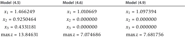
Table 1 Solutions results of models (4.5), (4.6), (4.9)

Model (4.5) Model (4.6) Model (4.9)

x1= 1.466249

x2= 0.9250464

x3= 0.4331181

maxz= 13.84631

x1= 1.010669

x2= 0.000000

x3= 0.000000

maxz= 7.074686

x1= 1.097394

x2= 0.000000

x3= 0.000000

Therefore, deterministic equality of CCSP model given in (4.1) can be found as fol-lows:

maxz= 7x1+ 2x2+ 4x3

4x1+ 4x2+ 6x3+ 1.645 %

4x2

1+ 8x22+ 12x23≤8

(4:9)

5x1+x2+ 6x3≤10.855

xj≥0 j= 1, 2, 3, 4

Model (4.9) has been solved by software Lingo 9.0and the results are listed in Table 1.

5. Conclusion

In this study, a new method is suggested for the solution of the deterministic equiva-lence of the CCSP. The main purpose of this article is to transform the chance-con-strained model into a deterministic model based on the Essen inequality. According to the Essen inequality, the estimation of the distance between the distribution of a sum of independent random variables and the normal distribution is less than or equal to

SLn. This study considers a stochastic optimization model with random technology

matrix in which the random variables are independent and follow a Gamma distribu-tion. Deterministic equality of these kinds of problems has been obtained via the sug-gested method. Furthermore, by adding a second constraint having normal distribution in the right-hand side value, a problem with two chance constraints has been obtained. In this problem, both cases that akjcoefficients have gamma and normal distributions

have been examined and for the solution of deterministic models Lingo 9.0 has been used.

As a result, the upper bounds of the chance constrained are derived by the Essen inequality and developed approximate deterministic equivalent of the model.

The solutions obtained by including the supremum distance defined by the Essen inequality in the model are shown clearly in the solutions results (4.5) and (4.6) in Table 1.

For large values of n, the solution results of the models having Gamma and normal distributions are closed to each other. This can be observed in Table 1 by examining the solution results (4.6) and (4.9). Here, it can be seen that coefficients of the objec-tive function and decision variables are very similar.

Author details

1_{Department of Medical Education, Faculty of Medicine, 06490, Bahçelievler, Ankara, Turkey}2_{Department of Statistics,}

Faculty of Science, 06100, Tandogan, Ankara, Turkey

Authors’contributions

All authors conceived of the study, participated in its design and coordination, drafted the manuscript, participated in the sequence alignment, read and approved the final manuscript.

Competing interests

The authors declare that they have no competing interests.

References

1. Charnes, A, Cooper, WW: Chance constrained programming. Manag Sci.6, 73_–79 (1959). doi:10.1287/mnsc.6.1.73 2. Symonds, GH: Deterministic solutions for a class of chance constrained programming problems. Oper Res.5, 495–512

(1967)

3. Kolbin, VV: Stochastic Programming. D. Reidel Publishing Company, Boston (1977)

4. Stancu-Minasian, IM: Stochastic Programming with Multiple Objective Functions. D. Reibel Publishing Company, Dordrecht (1984)

5. Hulsurkar, S, Biswal, MP, Sinha, SB: Fuzzy programming approach to multi-objective stochastic linear programming problems. Fuzzy Set Syst.88, 173–181 (1997). doi:10.1016/S0165-0114(96)00056-5

6. Liu, B, Iwamura, K: Chance constrained programming with fuzzy parameters. Fuzzy Set Syst.94, 227–237 (1998). doi:10.1016/S0165-0114(96)00236-9

7. Mohammed, W: Chance constrained fuzzy goal programming with right-hand side uniform random variable coefficients. Fuzzy Set Syst.109, 107_–110 (2000). doi:10.1016/S0165-0114(98)00151-1

8. Kampas, A, White, B: Probabilistic programming for nitrate pollution control: comparing different probabilistic constraint approximations. Eur J Oper Res.147, 217_–228 (2003). doi:10.1016/S0377-2217(02)00254-0

9. Yang, N, Wen, F: A chance constrained programming approach to transmission system expansion planning. Electric Power Syst Res.75, 171_–177 (2005)

10. Huang, X: Fuzzy chance constrained portfolio selection. Appl Math Comput.177, 500–507 (2006). doi:10.1016/j. amc.2005.11.027

11. Ağpak, K, Gökçen, H: A chance constrained approach to stochastic line balancing problem. Eur J Oper Res.180, 1098–1115 (2007). doi:10.1016/j.ejor.2006.04.042

12. Henrion, R, Strugarek, C: Convexity of chance constraints with independent random variables. Comput Optim Appl.41, 263–276 (2008). doi:10.1007/s10589-007-9105-1

13. Parpas, P, Rüstem, B: Global optimization of robust chance constrained problems. J Global Optim.43, 231_–247 (2009). doi:10.1007/s10898-007-9244-z

14. Xu, Y, Qin, XS, Cao, MF: SRCCP: a stochastic robust chance-constrained programming model for municipal solid waste management under uncertainty. Resour Conserv Recy.53, 352–363 (2009). doi:10.1016/j.resconrec.2009.02.002 15. Abdelaziz, FB, Masri, H: A compromise solution for the multiobjective stochastic linear programming under partial

uncertainty. Eur J Oper Res.202, 55–59 (2010). doi:10.1016/j.ejor.2009.05.019

16. Goyal, V, Ravi, R: A PTAS for the chance-constrained knapsack problem with random item sizes. Oper Res Lett.38, 161–164 (2010). doi:10.1016/j.orl.2010.01.003

17. Kall, P, Wallace, SW: Stochastic Programming. Wiley-Interscience Series in Systems and Optimization. John Wiley & Sons, Chicherster, UK (1994)

18. Prekopa, A: Stochastic Programming. Kluwer Academic Publishers, London (1995)

19. Hillier, FS, Lieberman, GJ: Introduction to Mathematical Programming. Hill Publishing Company, New York (1990) 20. Sakawa, M, Kato, K, Nishizaki, I: An interactive fuzzy satisficing method for multiobjective stochastic linear programming

problems through an expectation model. Eur J Oper Res.145, 665_–672 (2003). doi:10.1016/S0377-2217(02)00150-9 21. Sengupta, JK: A generalization of some distribution aspects of chance constrained linear programming. Int Econ Rev.

11, 287–304 (1970). doi:10.2307/2525670

22. Petrov, VV: Sums of Independent Random Variables. Springer-Verlag, New York (1975)

23. Feller, W: An Introduction to Probability Theory and Its Applications. John Wiley and Sons, Inc., New YorkII(1966) 24. Johnson, NL, Kotz, S: Distributions-I. A Wiley-Interscience Publication, New York (1970)

doi:10.1186/1029-242X-2011-108

Cite this article as:Atalay and Apaydin:Gamma distribution approach in chance-constrained stochastic

programming model.Journal of Inequalities and Applications20112011:108.

Submit your manuscript to a

journal and benefi t from:

7 Convenient online submission 7 Rigorous peer review

7 Immediate publication on acceptance 7 Open access: articles freely available online 7 High visibility within the fi eld

7 Retaining the copyright to your article