2019 International Conference on Artificial Intelligence and Computing Science (ICAICS 2019) ISBN: 978-1-60595-615-2
Classification of High Dimensional Small Sample Genetic Data by
Forward Maximum Likelihood Ratio Stepwise Logistic Regression
Li-hao WANG, Qiao-han CHU, Yi-ying ZHANG and Kun-ping ZHU
*Department of Mathematics, East China University of Science and Technology, Shanghai, China.
*Corresponding author
Keywords: Classification, Logistic regression,Likelihood ratio, Principal components.
Abstract. Analyzing genetic data has been one of the effective ways in early diagnosis of cancer. However, the method of machine learning usually needs the support of large data. For the small sample and with high dimensional genetic data, the accuracy of classification is generally not ideal by means of machine learning directly. This paper deals with the modeling of classification for high dimensional genetic data with only 62 samples. By extracting the principal components, it shows that the cumulative contribution rate of the first nine principal components can reach 80.73%, but the classification effect based on the principal components is not desirable. For the sake of reduction of the dimensions, the test of maximum Likelihood Ratio is applied for the selection of variables in logistic stepwise regression, which ensures that only the variables with significant influence on classification can enter the model. With the procedure, the final model fits well and is of good predicting performance.
Introduction
Data Information
The data to be analyzed comes from question A of 2010 National Post-Graduate Mathematical Contest in Modeling. The given data file contains the log2 intensity of the 2000 genes with highest minimal intensity (rows) of the 62 samples (columns), including 22 normal samples and 40 cancer samples. Based on the training data, the problem is to establish a classification model for the purpose of cancer prediction.
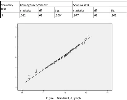
Fist, all the 2000 characteristics’ value are normally distributed. Due to the small sample data, we take K-S test into account. As shown in Table 1 of the third characteristic data for example, the Sig. is 0.2, which means the normality of the 3rd variable underSignificance level 0.05.For more intuitive, the Q-Q graph is given in figure 1, where x-axis stands for the observed value and y-axis stands for the expected standard value.
Table 1. Normality test.
Normality Test
Kolmogorov-Smirnova Shapiro-Wilk
statistics df Sig. statistics df Sig.
[image:2.612.100.510.238.560.2]3 .082 62 .200* .977 62 .302
Figure 1. Standard Q-Q graph.
Although there are 2000 characteristics, there is a strong correlation between them. Taking the first 100 variables as an example, the range of correlation is from -0.223 to 0.994. Thereby, we can understand the data information by extracting the principal components. The extraction result shows that the cumulative contribution rate of the first 2 principal components is 55.9%, and the cumulative contribution of the first 9 principal components reaches 80.73%. We try to classify according to the 9 principal components, but the practice shows thataccuracy of classification is not high by principal components.
Figure 2. Distribution of the two principal components.
Logistic Regression
In general, Logistic Regression [3,4] is a method to solve binary problems. Through estimating parameters of the logistic model to fit the data, it can predict the binary results. Conditions can be divided into “Yes” or “not”, they are often labeled as “1” or “0” as indicator variable. For instance, it can predict the probability of developing a certain disease (cancer), according to observed characteristics dependent on different people (various gene expression data). We suppose that x1, x2,
..., xn are n variables of different characteristics, y is the presence (y=1) or absence (y=0) of a certain
result and the p indicates the probability of presence (y=1). Then the following equation describes the relationships between different characteristics and p value [5]:
) ... ( 0 11
1
1
n nx
x
e
p
−β +β + +β+
=
(1)
where the coefficients βi are the parameters of the model associated with xi, including constant term
β0.We hereby use the gene related characteristics to substitute xi. Note that p is interpreted as the
probability of the dependent characteristics equaling the presence of the case rather than the absence. (e.g. if p=0.6, it tells that a patient have a 60% chance of having a malignant tumor ).
Generally, we consider that
otherwise p y
0
5 . 0 1
{ ≥
= (2)
which hereby means if p≥0.5 then the patient has cancer, otherwise the patient is healthy.
Estimation of Parameters
According to what has been supposed above, we suppose that l=βTx+β
0, where β= (β1, β2,..., βn)T. Then
from logistic function, we can get
l
e
l −
+ =
1 1 ) ( φ
(3)
Due to the fact that p indicates the probability of “1”, we can obtain that
y y
l l
x y
P = − 1−
)) ( 1 ( ) ( ) ; |
( β φ φ . And we suppose that there are m samples, then the likelihood function is
∏
∏
= − =−
=
=
m j y j j y j m j j j jl
l
x
y
P
L
1 1 ) ( ) ( ) ( 1 ) ( ) ( ()))
(
1
(
))
(
(
)
;
|
(
)
(
β
β
φ
φ
(4)
Logarithm to the formula (4), we get:
= − − + = m j j j j j l In y l In y L In 1 ) ( ) ( ) ( ) ( ))) ( 1 ( ) 1 ( )) ( ( ( )) (( β φ φ
(5)
where () () 0
β
β +
= T j
j x
l , j indicates the jth sample, y(j)indicates the real value of the jth sample and ((j)) l
φ
indicates the predict value of the jth sample.
If we put a negative sign in front of it, we should strive for minimize this function, which means that it can be used as a cost function:
=−
−
+
−
=
−
=
m j j j j jl
In
y
l
In
y
L
In
J
1 ) ( ) ( ) ( ) ()))
(
1
(
)
1
(
))
(
(
(
))
(
(
)
(
β
β
φ
φ
(6) )) ( 1 ( ) 1 ( )) ( ( ) ; ), (
( l y yIn l y In l
J
φ
β
=−φ
− − −φ
(7)Now we use gradient descent to calculate the parameters:
β β
β:= +∆ ; ∆β=-η∇J(β); βk:=βk+∆βk; k J β β η β ∂ ∂ − =
∆ k ( )
(8)
where βk indicates the kth characteristic coefficient; η indicates the learning rate to control the steps.
Because of φ'(l)=φ(l)(1−φ(l)), we can get that
= = − − = ∂ ∂ − − − − = ∂ ∂ m j j k j j m j j j j j j j k x l y l l y l y J 1 ) ( ) ( ) ( 1 ) ( ) ( ) ( ) ( ) ( )) ( ( ) ( ) ) ( 1 1 ) 1 ( ) ( 1 ( ) ( φ β φ φ φ β β (9)Therefore, the maximum likelihood estimation of the parameters is
= − + = m j j k j j x l y 1 ) ( ) ( ) ( kk
β
η
(φ
( ))β
:(10)
Likelihood Ratio Test
Basic principles: we start from a simple regression formula with only a constant term, then pick some of the variables which contribute most to the regression into the regression formula to minimize residual sum of squares and at the same time to avoid multi-collinearity.
We suppose that (X1,X2,...,Xn) are samples obtained from population ζ, (x1,x2,...,xn) are observed
value corresponding to the samples. The density function of population ζ is p(x,θ), θ∈Θ, Where
Θ=Θ0∪Θ1 indicates the value space of θ, and Θ0∩Θ1=∅, the test of parameter θ: H0:θ∈Θ0,
H1:θ∈Θ1, we take
) ( sup ) ( sup ) ,..., , ( 0 2 1 θ θ λ θ θ L L x x x n Θ ∈ Θ ∈
= (11)
as the statistic of the generalized likelihood ratio and call it likelihood ratio function [8].
)) ,..., , ( ( 2
- In λ x1 x2 xn (12)
which obey chi square distribution whose degree of freedom is 1 [10,11].
Analysis and Conclusion
We first use Z-score standardization to standardize all the characteristics by:
i i
S x x
z= i− (13)
We calculate the maximum likelihood estimation before and after considering this variable in the function and then put them into (13). We set a threshold for it, if it’s smaller than the threshold and if those variables pass the test with given confidence level, they can be taken into account. The analysis process is shown in Figure 3 as follows:
[image:5.612.105.507.254.357.2]rd M
Figure 3. Process of analysis.
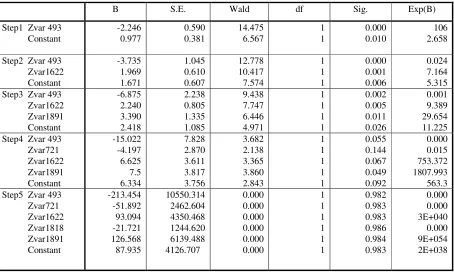
According to the steps given above, we have considered all the variables and finally 5 variables that meet the requirement are taken into account. They are 493rd, 721st, 1622nd, 1818th, 1891st variables.
The intermediate results of analysis are given in Table 2.
Table 2. Variables in the equation.
B S.E. Wald df Sig. Exp(B)
Step1 Zvar 493
Step1 Constant
-2.246 0.977 0.590 0.381 14.475 6.567 1 1 0.000 0.010 106 2.658
Step2 Zvar 493
Step1 Zvar1622
Step1 Constant
-3.735 1.969 1.671 1.045 0.610 0.607 12.778 10.417 7.574 1 1 1 0.000 0.001 0.006 0.024 7.164 5.315 Step3 Zvar 493
Step1 Zvar1622
Step1 Zvar1891
Step1 Constant
-6.875 2.240 3.390 2.418 2.238 0.805 1.335 1.085 9.438 7.747 6.446 4.971 1 1 1 1 0.002 0.005 0.011 0.026 0.001 9.389 29.654 11.225 Step4 Zvar 493
Step1 Zvar721
Step1 Zvar1622
Step1 Zvar1891
Step1 Constant
-15.022 -4.197 6.625 7.5 6.334 7.828 2.870 3.611 3.817 3.756 3.682 2.138 3.365 3.860 2.843 1 1 1 1 1 0.055 0.144 0.067 0.049 0.092 0.000 0.015 753.372 1807.993 563.3 Step5 Zvar 493
Step1 Zvar721
Step1 Zvar1622
Step1 Zvar1818
Step1 Zvar1891
Step1 Constant
[image:5.612.81.535.450.722.2]According to the calculation, the final regression function is:
) 935 . 87 568 . 126 721 . 1 2 -094 . 93 892 . 51 454 . 231
( 493 721 1622 1818 1891
1
1
+ +
+ −
− −
+
=
x x x x xe
y
(14)The result of classification is given in Table 3, which shows that the final regression function (14) can correctly classify the 62 samples with only 5 characteristics and is of 100% prediction accuracy. Although the model has perfectly fitted the data, there are still problems with this seemingly wonderful result according to related reference [12]. One of the most probable problems is that it’s over-fitting under some circumstances. Theoretically, further research for the method of forward stepwise likelihood ratio logistic regression is needed.
Table.3 Classification table.
Observed
Predicted
Yes or No Percentage Correct
0 1
Step 1 Yes or No 0
Step 1 Yes or No 1
Step 1 Overall Percentage
16 4
6 36
72.7 90.0 93.9 Step 2 Yes or No 0
Step 1 Yes or No 1
Step 1 Overall Percentage
19 4
3 36
86.4 90.0 88.7 Step 3 Yes or No 0
Step 1 Yes or No 1
Step 1 Overall Percentage
22 2
0 38
100.0 95.0 96.8 Step 4 Yes or No 0
Step 1 Yes or No 1
Step 1 Overall Percentage
22 1
0 39
100.0 97.5 98.4 Step 5 Yes or No 0
Step 1 Yes or No 1
Step 1 Overall Percentage
22 0
0 40
100.0 100.0 100.0
References
[1] J.D. Cohen et al., Science 10.1126 / science.aar3247 (2018).
[2] L. Qi and J. Shen, Construction of recurrence model of patients with hepatocellular carcinoma by gene mutation information in TCGA database combined with machine learning software RapidMiner, Chinese Journal of Liver Diseases (Electronic Version), 2018 10(3).
[3] Walker, S.H.; Duncan, D.B. (1967). “Estimation of the probability of an event as a function of several independent variables”. Biometrika. 54 (1/2): 167–178. doi:10.2307/2333860. JSTOR 2333860
[4] Cox, DR (1958). “The regression analysis of binary sequences (with discussion)”. J Roy Stat Soc B. 20 (2): 215–242. JSTOR 2983890.
[5] M. Hassan, M.A. Butt and M.Z. Baba, Logistic Regression Versus Neural Networks: The Best Accuracy in Prediction of Diabetes Disease, Asian Journal of Computer Science and Technology, ISSN: 2249-0701 Vol. 6 No. 2, 2017, pp. 33-42.
[6] Z. Zhou, Machine Learning [M], Beijing: Tsinghua University Press, 2016: 53-68.
[8] J. Liu, K. Zhu and Y. Lu, Applied Mathematical Statistics [M], Shanghai: East China University of Science and Technology Press, 2014: 95-98, 141-148.
[9] Hosmer, David W.; Lemeshow, Stanley (2000). Applied Logistic Regression (2nd ed.). Wiley. ISBN 978-0-471-35632-5.
[10]Cohen, Jacob; Cohen, Patricia; West, Steven G.; Aiken, Leona S. (2002). Applied Multiple Regression/Correlation Analysis for the Behavioral Sciences (3rd ed.). Routledge. ISBN 978-0-8058-2223-6.
[11]Allison, Paul D. “Measures of Fit for Logistic Regression”. Statistical Horizons LLC and the University of Pennsylvania.