http://dx.doi.org/10.4236/jst.2013.34019
Clustering in Wireless Multimedia Sensor Networks
Pushpender Kumar, Narottam Chand
Department of Computer Science and Engineering, National Institute of Technology, Hamirpur, India Email: [email protected], [email protected]
Received October 24, 2013; revised November 27, 2013; accepted December 4, 2013
Copyright © 2013 Pushpender Kumar, Narottam Chand. This is an open access article distributed under the Creative Commons At-tribution License, which permits unrestricted use, disAt-tribution, and reproduction in any medium, provided the original work is prop-erly cited.
ABSTRACT
Wireless Multimedia Sensor Networks (WMSNs) are comprised of small embedded audio/video motes capable of ex- tracting the surrounding environmental information, locally processing it and then wirelessly transmitting it to sink/base station. Multimedia data such as image, audio and video is larger in volume than scalar data such as temperature, pres-sure and humidity. Thus to transmit multimedia information, more energy is required which reduces the lifetime of the network. Limitation of battery energy is a crucial problem in WMSN that needs to be addressed to prolong the lifetime of the network. In this paper we present a clustering approach based on Spectral Graph Partitioning (SGP) for WMSN that increases the lifetime of the network. The efficient strategies for cluster head selection and rotation are also pro-posed as part of clustering approach. Simulation results show that our strategy is better than existing strategies.
Keywords: Wireless Multimedia Sensor Network; Clustering; Spectral Graph Partitioning; Eigenvector; Eigenvalue
1. Introduction
Recent developments in wireless communication and em- bedded technology have made the wireless sensor net- work (WSN) possible. Wireless sensor networks are con-stituted of large number of low-cost, low-power and less communication bandwidth tiny sensor nodes. The sensors, which are randomly deployed in an environment, are required to collect data from their surroundings, process the data and finally send it to the sink through multi hops [1]. Traditional WSNs collects the scalar data such as temperature, pressure, etc. and transmit it to the sink. WSN has potential to design many new applications for handling emergency, military and disaster relief opera-tions that require real time information for efficient coor-dination and planning [2].
Wireless multimedia sensor network (WMSN) uses cheap CMOS (Complementary Metal Oxide Semicon-ductor) camera and microphone sensors which can ac-quire multimedia information. WMSN consists of camera sensors as well as scalar sensors. Camera sensors can retrieve much richer information in the form of images or videos and hence provide more detailed and interesting data about the environment [3,4]. The multimedia con-tent has the pocon-tential to enhance the level of information collected, compared with scalar data. Multimedia content produces immense amount of data to transmit over
WMSN, which is limited in terms of power supply, com- munication bandwidth, memory, etc.
In a large scale network, if all the nodes have to com- municate their data to their respective destination, it will deplete their energy quickly due to the long-distance, large volume of data and multi-hopnature of the communication. This will also lead to network contention. The clustering is a standard approach for achieving efficient and scal- able control in these networks [5].
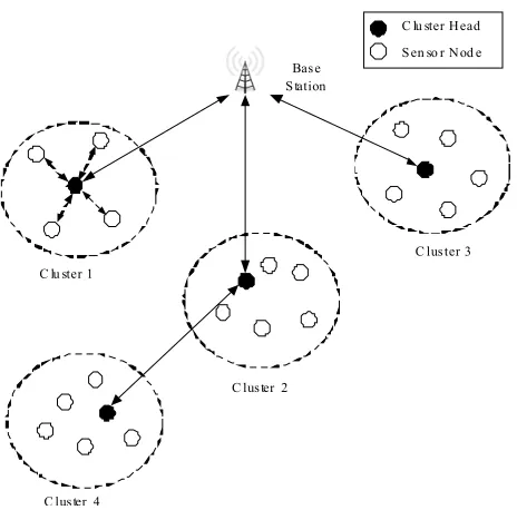
Clustering results in a number of benefits. It facilitates distribution of control over the network. It saves energy and reduces network contention by enabling locality of communication. Nodes communicate their data over short- er distances to their respective cluster head (CH). The cluster head aggregates these data into a smaller set of meaningful information. Not all nodes, but only the clus- ter heads need to communicate with their neighbouring cluster heads and sink/base station. Figure 1 shows the
clustering of nodes in a general WSN.
In this paper, we have utilized spectral graph partition- ing (SGP) technique based upon eigenvalues proposed by Fiedler to form clustering in WMSN [6]. SGP method has been used in many applications such as image segmenta- tion, social networks, etc. [7].
Base S tation
C lu ster 1
C luster 2
C luster 3 C lu ster Head S en so r Nod e
[image:2.595.58.290.81.310.2]C luster 4
Figure 1. Clustering of SNs in WSN.
The second highest eigenvalue of the Laplacian matrix corresponding to different eigenvectors, is used to parti-tion the graph into two parts. Within a cluster, a node with highest eigenvalue is selected as cluster head. In case of WMSN, large volume of sensed data is generated, therefore, such clustering can be utilized to reduce the volume and number of data transmissions through data aggregation. Simulation experiments have been perform- ed to evaluate the performance of proposed method and compare it with the existing technique.
The rest of the paper is organized as follows. Section 2 reviews the related work. General SGP strategy for clus-tering has been presented in Section 3. Section 4 de-scribes the use of SGP for WMSN. In Section 5 we pre-sent the results of performance evaluation of the method and Section 6 concludes the paper.
2. Related Work
The nodes are often grouped together into disjoint and mostly non-overlapping groups are called clusters. Clus- ters are used to minimize communication latency and im- prove energy efficiency. Leader of every cluster is often called the cluster head (CH) and generally has to perform more functions as compared to normal sensor node.
M. Qin et al. suggested voting-based clustering algo- rithm (VCA) [8] that enhances the criteria for cluster se- lection and combines load balancing consideration toge- ther with topology and energy information. VCA ad- dresses inefficient cluster formation using a voting scheme, which enables the nodes to exchange information about their local network view. This method assumes synchro- nization among the nodes. Similar to WCA [9], the time required for the nodes to gather information about all
other nodes depends on the network size and is not con- stant.
B. Elbhiri et al. [7] suggested spectral classification based on near optimal clustering in wireless sensor net-works (SCNOPC-WSN) algorithm. This algorithm deals with the clustering problem in WSN. Energy aware adap- tive clustering protocol is used for the bi-partitioning spectral classification and it guarantees robust clustering. SCNOPC-WSN also deals with the optimization of the energy dissipated in the network.
Banerjee and Khuller [10] suggested hierarchical clus-tering algorithm based on geometric properties of the wireless network. A number of cluster properties such as cluster size and the degree of overlap, which are useful for the management and scalability of the hierarchy, are also considered while grouping the nodes. In the propos- ed scheme, any node in the WSN can initiate the cluster formation process. Initiator with least node ID will take precedence, if multiple nodes started cluster formation process at the same time.
Bandyopadhyay and Coyle [11] proposed EEHC which is a distributed, randomized clustering algorithm for WSNs with the objective of maximizing the network lifetime. CHs collect the sensor reading in their individual clusters and send an aggregated report to the base station. Their technique is based on two stages—initial and extended.
In EEUC [12], the hot-spot problem in multihop net-works is solved using cluster with unequal size. CHs that are closed to the base station tend to die faster, because they relay much more traffic than remote nodes. Setting smaller cluster sizes to the close CHs preserves their en-ergy. Additional improvement for multihop networks is presented in [13], using a separation between the data gathering and aggregation task and the forwarding task.
Spectral graph partitioning algorithm partitions the graph using the eigenvectors of the matrix obtained from the graph. SGP obtains data representation in the low-di- mensional space that can be easily clustered. Eigenvalues and eigenvectors provide a penetration into the connecti- vity of the graph.
3. SGP for Cluster Formation
Spectral graph partitioning technique is based on eigen-values and eigenvector of the adjacency matrix of graph to partition the graph. The methods are called spectral, because they make use of the spectrum of the adjacency matrix of the data to cluster the points [14]. Spectral me-thods are widely applied for graph partitioning. Spectral graph partitioning is a powerful technique and also is being used in image segmentation and social network analysis. SGP divides the graph into two disjoint groups, based on eigenvectors corresponding to the second small- est eigenvalue of the Laplacian matrix [15].
the set of vertices (sensor nodes) and E represents the set of edges connecting these vertices. Each vertex is identi-fied by an index The edge between node
i and node j is represented by eij. The graph can be
rep-resented as an adjacency matrix. The adjacency matrix A of graph G having N nodesis the N × N matrix where the non-diagonal entry aij is the number of edges from node i
to node j, and the diagonal entry aii is the number of
loops at node i. The adjacency matrix is symmetric for undirectedgraphs [16].
1, 2, , .i N
j
The adjacency matrix A is defined as
1 edge weight between node and node 0 otherwise
ij
i A a
We also define degree matrix D for graph G. The de-gree matrix of a graph gives the number of edges be-tween node i to another node [17]. The degree matrix is a diagonal matrix which contains information about the degree of each node. It is helpful to construct the Lapla-cian matrix of a graph. The degree matrix D for G is a N
× N square matrix and is defined as
total weight of edges incident to node deg
0
ij
i D
The Laplacian matrix is formed from adjacency matrix and the degree matrix. The Laplacian matrix of the graph
G having N vertices is N × N square matrix and is repre-sented as
L D A
The normalized form of Laplacian matrix can be writ-ten as
i j
1 if and deg 0
1
, if and are adjacent deg deg
0 otherwise
j
i j
i j i j
The eigenvalues of matrix are denoted by
, 1, 2, ,
i i N
such that 12n
.
Laplacianmatrix has the property X X
where X is the
eigenvector of the matrix and λ is the eigenvalue of the matrix . Laplacian matrix plays important role in spectral graph theory. λ1 represents the number of sub-graphs in the network. The second smallest eigenvalue λ2 is referred to the algebraic connectivity and its corre-sponding eigenvector is usually referred to as the Fiedler Vector [14,18].
We choose the eigenvector values corresponding to the second highest eigenvalue λ2. Second highest eigenvalue (λ2) divides the graph into two subgraphs. G is divided into two subgraphs G and G , where G and are the set of vertices related to the new subgraphs. contains nodes corresponding to positive eigenvalues
and
G G
G contains nodes corresponding to negative ei-genvalues. The set of vertices is defined by
NNN
and
NN
where N G , N G and N G.
4. Cluster Formation in WMSN
SGP technique can be used for dividing the network into clusters. SGP has many advantages as compared to other clustering algorithms. SGP partitions the graph on the basis of eigenvalues and eigenvector adjacency matrix. If the graph is partitioned into more than two subgraphs, apply SGP technique recursively. These properties make SGP technique a better option for multimedia data clus-tering where large volume of data is transmitted between nodes and CH.
In our proposed method, clustering of WMSN has been done on the basis of Spectral Graph Partitioning technique [19]. Each node sends short message to sink which contains the location information of the node. On the basis of this information, the sink constructs the ad-jacency matrix and degree matrix and then constructs the Laplacian matrix. The eigenvector corresponding to sec-ond smallest eigenvalue (called Fiedler Vector) is used to partition the WMSN. The location of each node may be found by GPS or any other localization method [18,20].
4.1. Steps for Clustering
1) Construct a graph G of the given sensor network. 2) Construct the normalized Laplacian matrix as
i j
1 if and deg 0 1
,
i j
deg
if and are adjacent deg deg 0 otherwise j i j i j
where i is the degree of node i
3) From the Laplacian matrix of the graph com-pute the eigenvalues and eigenvector of Laplacian ma-trix.
4) Select the second smallest eigenvalue λ2 of Lapla-cianmatrix .
5) Choose eigenvector value corresponding to the ei-genvalue λ2.
Divide the graph G into two subgraphs G and G
,
where G contains nodes corresponding to positive ei- genvalues and G, contains nodes corresponding to ne- gative eigenvalues.
eigen-values of the nodes. Table1 shows the two partitions/
clusters for a given graph shown in Figure2. After first
iteration cluster 1 contains all the nodes with positive eigenvector values and another cluster 2 contains nodes having negative eigenvector values. Cluster 1 has five nodes with positive value of eigenvector and the nodes are A, B, C, D and F. Cluster 2 has five nodes that have negative eigenvector values and the nodes are E, G, H, I and J.
Only two clusters are formed in first iteration. The larger size clusters can be further divided into two dif-ferent clusters by applying the algorithm recursively. This process continues until maximum intra-node dis-tance within a cluster is less than R 2 2 where R is the transmission range of the sensor node. When intra- node distance is remaining R 2 2 two nodes in neigh-
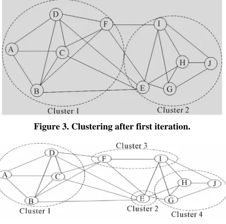
bouring clusters can communicate in one hop. After ap- plying the algorithm recursively, the given network is divided into four clusters as shown in Figure3. Table2
shows the formed cluster after first iteration.
It has been observed that both the clusters have higher intra-node distance than R 2 2, so apply the algorithm to both the clusters. After applying the algorithm cluster 1 is portioned into two different clusters. This algorithm is also applied to cluster 2 of Figure3.
Thus the whole network is divided into four clusters as shown in Figure 4. Table3 shows different nodes pre-
sent in the each cluster
4.2. Cluster Head Election
The clustering algorithm divides the whole network into clusters. The next step is election of cluster head for each cluster. As per the property of SGP, the least eigenvector value of node signifies that the node is well connected to the other nodes within the cluster as well as it is con-nected to cluster [21].
For initial cluster head election, we chose the least ei-genvector value among the nodes within cluster, Table4
represents the eigenvector values of the cluster and Ta- ble5 shows the elected cluster heads in different clusters
on the basis of eigenvector values. Therefore, we com- pare the eigenvector values of the cluster and choose the
A
B C D
E
F I
J H
[image:4.595.313.535.86.306.2]G
Figure 2. Given graph.
Figure 3. Clustering after first iteration.
Figure 4. Network after clustering.
Table 1. Eigenvector table and clustering of given network.
Node Degree Eigenvalue Eigenvector (for λ2)
A 3 0 0.3235
B 5 0.2448 (λ2) 0.3155
C 5 0.8987 0.3155
D 5 1.076 0.3155
E 7 1.200 −0.0190
F 5 1.200 0.1592
G 4 1.250 −0.3853
H 4 1.263 −0.3853
I 5 1.378 −0.3293
[image:4.595.306.540.348.577.2]J 3 1.488 −0.4070
Table 2. Initial clusters of network.
Cluster No Nodes Eigenvalue
Cluster 1 A, B, C, D, F Positive
Cluster 2 E, G, H, I, J Negative
Table 3. Final clusters for the network.
Cluster Number Nodes
Cluster 1 A, B, C, D
Cluster 2 E
Cluster 3 F, I
[image:4.595.62.280.608.723.2]Table 4. Clustering after second iteration.
Node Cluster Initial Eigenvalue Eigenvector (for λ
2) Cluster
A 0 −0.7071
B 1.000 (λ2) −0.00001
C 1.2500 −0.00001
D 1.2500 −0.00001
Cluster 1
E
C L U S T E R
1 1.5000 0.7071 Cluster 2
F 0 0.7475
I 0.7257 (λ2) 0.4101
Cluster 3
G 1.330 −0.3017
H 1.330 −0.3017
J
C L U S T E R
2 1.607 −0.3017
[image:5.595.56.288.329.415.2]Cluster 4
Table 5. Elected cluster heads.
Cluster Number Eigenvector Cluster Head
Cluster 1 0.7071 A
Cluster 2 0.7071 E
Cluster 3 0.7475 F
Cluster 4 0.3017 G
least eigenvector node as a cluster head.
Cluster Head Least Eigenvector
Figure5 shows the flow chart for cluster head
selec-tion and rotaselec-tion.
Figure6 shows the elected cluster heads for different
clusters.
Cluster head rotation must take place when residual energy (Eres) of the cluster head node falls below the
threshold value (Eth). The present cluster head declares
the election process by sending a message that contains its Eres to all the cluster members. The cluster members
whose residual energy is greater than Eres responds to this
message by sending the residual energy to the cluster head.
The new cluster head is elected based upon CH Can-didacy Factor (CF) defined as
i res i
i
E CF
D
where is the residual energy of node i, Di is the
distance between node i and current cluster head. If
i res
E
ch
ch,
i ch i ch
D x x y yi
A node with highest value of CF is elected as next cluster head.
5. Performance Evaluation
In this section the performance of SGP has been evalu-ated through simulation. The simulation has been per-formed in Matlab2013a. The performance of SGP proto-col is compared with HEED [22]. The performance met-rics include percentage of nodes acting as cluster heads and ratio of single node cluster and network lifetime.
Ratio of single node cluster indicates that the ratio of number of clusters having single nodes to the total num-ber of clusters. If the ratio of single node clusters in the network is high, it may lead to early energy dissipation.
Figure 7 illustrates the percentage of cluster with
more than one node. High single node cluster (the cluster head) may lead to reduce the network lifetime. Single node cluster arise when a node is forced to represent it-self. The figure shows that HEED produces a higher per- centage of non-single node clusters than the SGP.
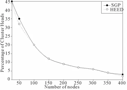
Percentage of nodes acting as cluster head describes the fraction of total sensor nodes in percentage, acting as cluster head in the sensing field. In WMSN, smaller per-centage of nodes should act as CH, creating a cluster which has enough number of sensor nodes (cluster mem- bers). High values indicate that numbers of clusters are present in the network with small size of clusters.
Figure8 shows the percentage of cluster heads select-
ed by both HEED and SGP (for different number of nodes) are identical.
6. Conclusion
This paper has proposed an approach to deal with the
Start cluster head selection and rotation process
Cluster head selection or rotation
Rotation
Selection
Highest eigenvector value
Highest current energy
where Di is the distance
i res cur
i
E E =
D
2 2
i ch i ch i
D = (x - x ) + (y - y ) Cluster Head = Least Eigenvector
x y and
x yi, i
are the location coordinates of [image:5.595.308.539.525.708.2]Figure 6. Election cluster heads of given graph.
Figure 7. Percentage of non-single node cluster.
Figure 8. Percentage of selected cluster heads.
clustering problem in a given wireless multimedia sensor network. We have explained the details of the proposed clustering algorithm. It divides the network into two clu- sters and partitions the network till we get the clustering, where nodes in neighbouring clusters can communicate using single hop. A cluster head elections technique bas- ed on eigenvector has also been proposed. Simulation re- sults show that our proposed algorithms perform better than those HEED algorithms.
REFERENCES
[1] F. Akyldiz, W. Su, Y. Sankarasubramaniam and E.
Cay-irci, “Wireless Sensor Networks: A Survey,” Computer
Networks, Vol. 38, No. 4, 2002, pp. 393-422.
[2] S. Taruna and M. R. Tiwari, “An Event Driven Energy Efficient Data Reporting System for Wireless Sensor Net- works,” Vol. 2, No. 2, 2013, pp. 70-75.
[3] I. F. Akyildiz, T. Melodia and K. R. Chowdhury, “A Sur- vey on Wireless Multimedia Sensor Networks,” Compu-
ter Networks, Vol. 51, No. 4, 2007, pp. 921-960.
[4] P. Kumar and N. Chand, “Clustering in Wireless Multi- media Sensor Networks Using Spectral Graph Partition- ing,” International Journal of Communication, Network
and System Sciences, Vol. 6, No. 3, 2013, pp. 128-133.
[5] M. Demirbas, A. Arora, V. Mittal and V. Kulathumani, “A Fault-Local Self-Stabilizing Clustering Service for Wire- less Ad Hoc Networks,” IEEE Transactions on Parallel
and Distributed Systems, Vol. 17, No. 9, 2006, pp. 912-
922.
[6] B. Auffarth, “Spectral Graph Clustering,” Course Report. http://wwwlehre.inf.uos.de/~bauffart/spectral.pdf
[7] B. Elbhiri, S. El Fkihi, R. Saadane and D. Aboutajdine, “Clustering in Wireless Sensor Network Based on Near Optimal Bi-partitions,” 6th EURO-NF Conference on Next
Generation Internet (NGI), 2010, pp. 1 -6.
[8] M. Qin and R. Zimmermann, “VCA: An Energy Efficient Voting Based Clustering Algorithm for Sensor Networks,”
Journal of Universal Computer Science, Vol. 13, No. 1,
2007, pp. 87-109.
[9] M. Chatterjee, S. K. Das and D. Turgut, “WCA: A Weight- ed Clustering Algorithm for Mobile Ad hoc Networks,”
Journal of Cluster Computing (Special Issue on Mobile
Ad hoc Networks), Vol. 5, No. 2, 2002, pp. 193-204.
[10] S. Banerjee and S. Khuller, “A Clustering Scheme for Hi- erarchical Control in Multi-Hop Wireless Networks,” IEEE INFOCOM, 2001, pp. 1028-1037.
[11] S. Bandyopadhyay and E. Coyle, “An Energy Efficient Hierarchical Clustering Algorithmfor Wireless Sensor Net- works,” 22nd Annual Joint Conference of the IEEE Com-
puter and Communications Societies (INFOCOM), Vol. 3,
2003, pp. 1713-1723.
[12] C. Li, M. Ye, G. Chen and J. Wu, “An Energy Efficient Unequal Clustering Mechanism for Wireless Sensor Net- works,” 2nd IEEE International Conference on Mobile
Ad-hoc and Sensor Systems (MASS), 2005, pp. 125-132.
[13] Y. He, Y. Zhang, Y. Ji and S. X. Shen, “A New Energy Efficient Approach by Separating Data Collection and Data Report in Wireless Sensor Networks,” International
Conference on Communications and Mobile Computing,
2006, pp. 180-192.
[14] A. Bertrand and M. Moonen, “Distributed Computation of the Fiedler Vector with Application to Topology Infer- ence in Ad Hoc Networks,” Internal Report KU Leuven ESAT-SCD, 2012.
[15] Laplacian Matrix Wikipedia.
http://en.wikipedia.org/wiki/Laplacian_matrix [16] Adjacency Matrix Wikipedia.
[image:6.595.65.281.405.557.2]http://en.wikipedia.org/wiki/Degree_matrix
[18] A. Savvides, C. Han and M. B. Srivastva, “Dynamic Fine- Grained Localization in Ad Hoc Networks of Sensors,”
7th International Conference on Mobile Computing and
Networking (MOBICOM), 2001, pp. 166-179.
[19] D. Lu, N. Nan and X.-X. Huang, “Clustering Based Spec- trum Allocation Scheme in Mobile Ad Hoc Networks,”
Bulletin of Advanced Technology Research (BATR), Vol.
5, No. 12, 2011, pp. 37-41.
[20] N. Bulusu, J. Heidemann and D. Estrin, “GPS-Less Low Cost Outdoor Localization for Very Small Devices,” IEEE
Personal Communication Magazine, Vol. 7, No. 5, 2000,
pp. 28-34.
[21] A. Savvides, C. Han and M. B. Srivastva, “Dynamic Fine- Grained Localization in Ad Hoc Networks of Sensors,”
7th International Conference on Mobile Computing and
Networking (MOBICOM), 2001, pp. 166-179.