Munich Personal RePEc Archive
Locational signaling and agglomeration
Berliant, Marcus and Yu, Chia-Ming
Washington University in St. Louis
29 July 2010
Online at
https://mpra.ub.uni-muenchen.de/24155/
Locational Signaling and Agglomeration
∗
Marcus Berliant
†and Chia-Ming Yu
‡July 29, 2010
Abstract: Agglomeration can be caused by asymmetric information and a locational signaling effect: The location choice of workers signals their pro-ductivity to potential employers. The cost of a signal is the cost of hous-ing at a location. When workers’ marginal utility of houshous-ing is negatively correlated with their productivity, skill-biased technological change causes a core-periphery bifurcation where the agglomeration of high-skill workers eventually constitutes a unique stable equilibrium. When workers’ marginal utility of housing and their productivity are positively correlated, skill-biased technological improvements will never result in a core-periphery equilibrium. Location can at best be an approximate rather than a precise sieve for high-skill workers. (JEL Classifications: D51; D82; R13)
Keywords: Agglomeration; Adverse Selection; Asymmetric Information; Locational Signaling
∗We thank Karl Dunz, Yasuhiro Sato, participants at the 2009 North American
Meet-ings of the Regional Science Association International, and participants at the spring 2009 Midwest Economic Theory meetings for comments. The second author acknowledges fi-nancial support from the Center for Research in Economics and Strategy (CRES) at the Olin Business School, Washington University in St. Louis. The authors retain responsi-bility for the contents of this paper.
†Department of Economics, Washington University, Campus Box 1208, 1 Brookings
Drive, St. Louis, MO 63130-4899. Phone: (1-314) 935-8486, Fax: (1-314) 935-4156, e-mail: [email protected]; and Division of the Humanities and Social Sciences, California Institute of Technology.
‡Department of Economics, Washington University, Campus Box 1208, 1 Brookings
1
Introduction
As shown in Baum-Snow and Pavan [2009], US wages were more than 30
percent higher in metropolitan areas with over 1.5 million inhabitants than
in rural areas in the year 2000. Furthermore, their model indicates that
ability sorting and returns to experience across locations are crucial elements
in explaining the wage premium in large cities. Glaeser and Mare [2001] show
that sorting on human capital accounts for about one-third of the city-size
wage gap in the US. Moreover, Gould [2007] demonstrates that migration of
high-skill workers is important in justifying the urban productivity premium,
that is amplified by steeper experience profiles in urban areas. These analyses
suggest that workers signal their skill and experience using their locations.
One natural question is: How can we empirically distinguish locational
signaling effects from agglomeration externalities? Agglomeration
external-ities and spillovers are widely analyzed in the literature, for example,
Hen-derson [1986], HenHen-derson et al. [1995], Glaeser et al. [1992], and Feldman
and Audretsch [1999]. Under the framework of agglomeration externalities,
an increase in the ratio of high-skill labor in one region causes more than
a proportional increase in the average real wage (or an increase in labor’s
marginal product). This gives us a clear empirical macro contrast between
signaling and agglomeration externality models. The growth of urban labor
productivity predicted by our signaling model is scale free (independent of
population) whereas that growth rate for agglomeration externality models is
not. When the growth rate in high-skill labor’s productivity is independent of
high-skill urban population, our signaling viewpoint is supported; otherwise,
the high-end productivity data supports the existence of an agglomeration
externality. As shown in Figure 1, a regression of average per capita GDP
growth rate on average population for 366 U.S. metropolitan areas (from 2001
0.5 1 1.5 2
Population HmillionsL
-0.02 -0.01 0.01 0.02 0.03 0.04 0.05
[image:4.612.139.453.100.254.2]GDP growth
Figure 1: Average per capita GDP growth rate for 366 U.S. metropolitan areas, 2001–2008. Source: U.S. Bureau of Economic Analysis.
0.013−0.00005∗(average metropolitan population), which suggests that the growth of metropolitan GDP is scale free and supports our signaling
view-point.1
Households’ private information includes their productivity, which varies
among individuals. When locations can possibly reveal workers’
productiv-ities, it is natural to ask why in practice some locations are attached to a
signal for high productivity of workers, while others are not. For example,
fashion designers in Milan, software programmers in Seattle, entertainers in
1Bode [2004] also shows that the estimated productivity effects of density almost
Hollywood, financiers on Wall Street, or high-tech workers in Silicon Valley
can be viewed as having a higher productivity than do workers in the same
field in other locations. These observations could be due to learning from
other workers, or interaction with R&D in these locations; however, they
could also be due to a locational signaling effect. Many tools are used to
sig-nal workers’ abilities since information about workers’ skill is very important
to firms and workers, for example: college diplomas, professional certificates,
and academic alliance memberships.2 It is interesting to examine how
high-skill workers can use locational agglomeration to distinguish themselves from
other workers, and how effective location can be as a reference for workers’
productivity.3
Berliant and Kung [2010] analyze how asymmetric information causes
ag-glomeration. Using a screening model, they show that workers can
agglomer-ate and be sorted by skill in equilibrium due to asymmetric information in the
labor market. Though it seems intuitive that both signaling and screening
can explain sorting by human capital and the significant wage premium in
large cities, one major difference between them is in the equilibrium sorting
patterns: In the screening model, since contracts are offered first, separation
of types by contract instead of location can occur, and thus, any distribution
of workers constitutes an equilibrium. Even considering stability, equilibrium
patterns are not narrowed down much. In contrast, for the signaling model,
separation of types can only occur by choice of location, not by choice of
con-tract. Thus, equilibrium narrows things down quite a bit. Furthermore, since
in reality it is rare to see complete sorting on location, the incomplete sorting
result in our signaling model is more persuasive than the screening model in
2In urban economics, for example, there is the UEA.
3Glaeser and Saiz [2003] also examine the incentive for people to agglomerate around
predicting equilibrium locational sorting patterns in workers’ productivity.
This paper answers the question: When there is asymmetric information,
does stratification emerge in equilibrium due to the signaling value of the
choice of location? The shadow cost of location, and thus of the signal, is
the price of housing in a region.
Krugman [1991a] and New Economic Geography (NEG) models adopt
in-creasing returns to scale to explain the agglomeration of manufacturing firms
in one region. When transportation cost is decreased as transportation
tech-nology is improved, a core-periphery pattern is more likely in equilibrium.
However, Pines [2001] points out that the NEG model ignores land
mar-kets, and thus omits the influence of housing prices on households’ location
decisions, which is the focus of our model. Many economic agglomeration
phenomena in reality cannot be satisfactorily explained by increasing returns
to scale. That is, there is a need to offer economic explanations other than
increasing returns to scale in explaining the agglomeration of industries
with-out increasing returns. A signaling incentive potentially fills this need. It is
natural to ask: Is a core-periphery configuration more likely to constitute an
equilibrium when there are no increasing returns to scale in production, but
rather asymmetric information?
In contrast to aggregate uncertainty discussed in Berliant and Yu [2009],
idiosyncratic uncertainty (individual-specific information) is the source of
asymmetric information in this paper. A model with two regions and two
types of workers, with high and low productivity, is analyzed in this
pa-per. Workers are mobile across regions while differences in regional wages
and housing rents determine their migration incentives. When workers’
mar-ginal utility of housing is negatively correlated with their productivity, as
shown in Figure 8, there are at least three equilibria: a completely
regions, and two partially stratified equilibria (or say core-periphery
equi-libria) where high-productivity workers are agglomerated in one region, but
low skill workers are not. When the difference in workers’ productivities is
small, the completely symmetric equilibrium is stable; when the difference in
workers’ productivity is large enough, the completely symmetric equilibrium
becomes unstable. In that case, there is no stable equilibrium. The partially
stratified equilibria are always stable. On the other hand, when workers’
mar-ginal utility of housing is positively correlated with workers’ productivity, as
shown in Figure 9, there always exists a completely symmetric equilibrium
but there are no core-periphery equilibria. The completely symmetric
equi-librium is stable when the difference in workers’ productivities is not large.
When the difference in productivities is very large, the completely symmetric
equilibrium is unstable.
For example, though a higher wage for workers in the fashion
indus-try in Milan attracts workers in an alternative region to migrate to Milan,
due to a larger aggregate housing demand, there will be a higher housing
rent in Milan to offset workers’ migration incentives. As shown in Figure 2,4
when high-productivity workers have a lower marginal utility of housing than
low-productivity workers, the utility cost of signaling for high-productivity
workers is lower than the utility cost of signaling for low-productivity
work-ers at the core-periphery equilibrium. Therefore, for a given wage premium
in Milan, there is a long-run stratified equilibrium such that all the
high-productivity workers agglomerate in Milan while the low-high-productivity
work-ers reside in both Milan and the alternative region. When high-productivity
workers have a higher marginal utility of housing than low-productivity
work-ers, as shown in Figure 3, the signaling cost for high-productivity workers is
higher than that for low-productivity workers under any core-periphery
con-4We shall explain the figures introduced here in detail later in the paper. This is a
figuration. This intuition is verified in this paper, which suggests a potentially
testable implication of our model, namely the prevalence of agglomeration of
high-skill workers as a function of the correlation of skill and marginal utility
of housing.
Notice that, in either a stratified or a symmetric equilibrium, no region
is fully occupied by high-productivity workers alone. That is, there is no
completely segregated equilibrium, but a semi-pooled equilibrium may exist.5
On the other hand, there is always a completely pooled equilibrium in our
model. Therefore, it is only possible to ensure that any worker who does not
reside in Milan is a low-productivity worker. For every worker in Milan, it is
impossible to guarantee that his/her productivity is high in any equilibrium.
This observation indicates that location is at best an approximate instead of
a precise sieve for high-productivity workers.
Furthermore, if we consider a continuous increase in high-skill workers’
productivity relative to that of low-skill workers, a core-periphery
bifurca-tion is present (Figure 8), even if there are no increasing returns to scale in
production and knowledge spillovers. In other words, the agglomeration of
high-productivity industries can be attributed to the existence of a locational
signaling effect. Since, intuitively, increasing returns to scale in fashion
de-sign seems bizarre, the agglomeration of fashion industries in Milan can be
explained from a signaling viewpoint.6
Signaling cost in our model is determined by housing prices, and housing
prices are different for different distributions of workers. In contrast with
most signaling models where the marginal signaling cost is exogenous, i.e.,
Spence [1973], Wilson [1977], Grossman [1981], and Rothschild and Stiglitz
5The core-periphery equilibrium in this paper corresponds to a semi-pooling equilibrium
where some types of senders choose the same signal (location) and other types choose different signals (locations).
6We do not claim that all agglomerations of high skill workers result from signaling.
[1976], the marginal signaling cost is endogenous in our paper. That is,
signaling cost affects workers’ migration incentives, and after their migration,
the distribution of workers’ types further influences the signaling cost. We
explore the question: Does the interaction between migration and marginal
signaling cost yield a separated equilibrium? The same type of endogeneity
also holds in cheap-talk models like Crawford and Sobel [1982] and
Austen-Smith and Banks [2000].
In what follows, our model is introduced in Section 2. Additionally,
nec-essary and sufficient conditions for the existence of stable core-periphery
equilibria and for the stability of integrated equilibria are presented.
Sev-eral numerical examples and related welfare analyses are offered in Section
3. Conclusions are in Section 4. An appendix contains the proof of the main
result.
2
Model
There are two regions k ∈ K ≡ {x, y} with the same land endowment ¯s. There are two types of mobile workers i ∈ N ≡ {H, L} with exogenous populations nH, nL
∈ R++, respectively, where the productivity of H-type
workers is higher than that ofL-type workers. H-type (L-type) workers can
be interpreted as high-skill (low-skill) workers, or can be interpreted as
ex-perienced (novice) workers. With the second interpretation, the appearance
of a stratified equilibrium implies that returns to experience are important
in explaining the city size wage premium.
Throughout this paper, workers’ type is indexed by a superscript and
location is indexed by a subscript. The (endogenous) population of i-type
workers living in k is denoted by ni
k, and the (exogenous) aggregate popu-lation in the model is n = nH +nL. Firms cannot recognize any worker’s
work-ers’ types over the two regions and can infer the probability of a worker’s
type using his/her location. Utility is quasilinear. Let si k, z
i
k be each i-type worker’s house size and the consumption of composite goods in region k,
i ∈ N, k ∈ K, respectively. Let rk denote the rent per unit of housing and let wk denote the worker’s wage in k, k ∈ K. Each worker is endowed with one unit of labor. The rents are collected and consumed by households, each
of whom is endowed with ei
k units of housing in k, i ∈ N, k ∈ K. Notice that nHeH
k +nLeLk = ¯s, k ∈ K. Letting ϕik ≡ (sik, zki), i ∈ N, k ∈ K, the optimization problem for H-type workers in regionk, k ∈K, is7
max uHk(ϕ H k) =z
H k −
α sH k s.t. rksHk +z
H
k ≤wk+rxexH +ryeHy , (1)
sH k, z
H
k ∈R+;
whereas the optimization problem for L-type workers in k is
max uLk(ϕ L k) =z
L k −
β sL
k s.t. rksLk +z
L
k ≤wk+rxexL+ryeLy, (2)
sL
k, zkL ∈R+.
Assume that α, β > 0. Either α > β holds, which implies that workers’
marginal utility of housing is positively correlated with productivity, orα < β
holds, implying that workers’ marginal utility of housing and productivity
are negatively correlated.8
7Except for asymmetric information, our model satisfies all the assumptions of
Star-rett’s [1978] theorem. That is, asymmetric information is the only source of agglomeration in this model.
8Whenα=β, the signaling cost is the same for both types of workers who thus have the
To simplify the analysis, assume that each worker inelastically supplies
one unit of labor, so we need not be concerned about monitoring and
vol-untary participation constraints. Every firm hires one worker at most. Each
firm can adopt a high type technology together with a H-type labor to
pro-duce YH, or adopt a low type technology together with a L-type labor to
produce YL, where 0 < YL < YH. The corresponding profit in k is YH−w k and YL−wk, respectively, k ∈K. When any firm adopts a high type tech-nology with a L-type worker, the output is zero. On the other hand, when a
firm adopts a low type technology and a H-type worker, the output is YL,
which is lower than YH. That is, no firm would prefer to adopt a technology
that is incompatible with the type of the hired worker. Firms maximize their
expected profit; their equilibrium behavior in choosing technology will be
ex-plained later. Every firm or worker is so small that he/she cannot influence
competitive market prices. Furthermore, assume that there is free entry of
firms, and thus, every firm earns zero expected profit in equilibrium. Finally,
workers choose locations to maximize their utilities, including the
considera-tion that firms can possibly learn about workers’ types only from observing
their locations.9
To extract the influence of signaling effects, assume that there is no
com-muting; that is, workers can work only in the place where they live. In other
words, this is a regional, not city, model. However, H-type andL-type
work-ers are allowed to migrate to earn a higher utility.10 Denote ρH (ρL) as the ratio of H-type (L-type) workers in the world living in x, and thus 1−ρH (1−ρL) is the ratio of all H-type (L-type) workers living iny. The
popula-equilibrium. That is, givenα=β, either there are an infinite number of equilibria (when
YH−YL is small) or there is no long-run equilibrium (whenYH−YL is large), which is not a case of interest.
9Since the agents are competitive in the housing market, they cannot do anything to
attract high-skill workers and increase their housing rental income.
10WhenH-type workers are mobile butL-type workers are immobile, there are similar
tion in x and y, given (ρH, ρL), can be expressed as n
x ≡ρHnH +ρLnL and
ny ≡(1−ρH)nH + (1−ρL)nL, respectively.
To characterize locational signaling effects, the market process is given as
follows. First, each firm hires a worker without knowing his/her productivity.
Though firms do not know each worker’s type, suppose that firms do not
misperceive; that is, they know the actual equilibrium proportion of H-type
workers in each region and thus have a common distribution over a worker’s
type conditional on his/her equilibrium location. Then, since there is a free
entry of firms, each firm in a region pays its worker a wage according to the
expected profit in the region. After learning the type of worker that the firm
hires, the firm chooses its production technology to maximize ex post profit
or minimize ex post loss. A mixed adoption of technology is assumed not
available for firms.11
Note that given (ρH, ρL), since there is free entry of firms, each firm earns
zero expected profit. Thus, the wages for every worker in region x and y
are12
wx(ρH, ρL) = 1
nx
(ρHnHYH +ρLnLYL), (3)
11Surely, changing the specified market process can change the results of our model.
For example, when firms are assumed to choose their technology before knowing workers’ type, the chosen technology must be the same for all firms in one region (since there is no difference between firms in the same region). Moreover, given workers’ distribution is not completely symmetric, when the high technology is chosen in one region in equilibrium, the other region will choose the low technology. Since theH-type (L-type) workers can be hired only in the region adopting the high (low) technology, a core-periphery equilibrium is immediate for any not-completely symmetric initial distribution of workers. Actually, this setting is more like a screening model as analyzed in Berliant and Kung [2010], instead of a signaling model. In addition, when firms pay the wage after they know workers’ type, there is no need for workers to use locational signaling. Therefore, the market process specified here is more appropriate in presenting a story for signaling effects than alternative assumptions.
12The main purpose of this paper is to characterize agglomeration across regions, instead
wy(ρH, ρL) = 1
ny
[(1−ρH)nHYH + (1−ρL)nLYL]. (4)
Let us temporarily leave workers’ mobility aside. Short-run equilibrium is
defined as a competitive market equilibrium, given a population distribution
over the two regions.
Definition 1 (Short-Run Equilibrium)
(ϕH∗
k , ϕLk∗, w∗k, rk∗)k∈K constitutes a short-run equilibrium if, given an arbitrary (ρH, ρL), workers choose optimal consumptions, firms make competitive wage
offers for the distribution of workers, and the housing and the composite good markets in each region clear. That is:
(a) ui
k(ϕik∗)≥uki(ϕik), for allϕik ∈R2+ satisfying rksik+zik≤wk, ∀i∈N,
k ∈K; (b) w∗
x=
1
nx(ρ
H∗nHYH +ρL∗nLYL), and
w∗
y = n1y[(1−ρ
H∗)nHYH + (1−ρL∗)nLYL];
(c) ρH∗nHsH∗
x +ρL∗nLsLx∗ =ρH∗nHeHx +ρL∗nLeLx = ¯s, (1−ρH∗)nHsH∗
y +(1−ρL∗)nLsLy∗ = (1−ρH∗)nH eHy +(1−ρL∗)nLeLy = ¯s, (ρH∗zH∗
x + (1−ρH∗)zyH∗)nH + (ρL∗zxL∗+ (1−ρL∗)zLy∗)nL =nHYH +nLYL.
The short-run equilibrium, by Walras’ law, is determined by conditions
(a), (b), and the first two (or any two) equalities in (c). Recalling that
nx ≡ ρHnH +ρLnL and ny ≡ (1−ρH)nH + (1−ρL)nL, and letting Yx ≡
ρHnHYH +ρLnLYL and Y
y ≡ (1−ρH)nHYH + (1−ρL)nLYL, Theorem 1 shows that the short-run equilibrium exists and is unique.
Theorem 1 For each(ρH, ρL)∈[0,1]×[0,1], there exists a unique short-run
equilibrium, where
sH∗
x =
√
αs¯
√
αρHnH +√βρLnL, s H∗
y =
√
αs¯
√
α(1−ρH)nH +√β(1−ρL)nL, (5)
sL∗ x =
√
βs¯
√
αρHnH +√βρLnL, s L∗ y =
√
βs¯
√
zH∗
x =
eH x(
√
αρHnH +√βρLnL)2
¯
s2 +
eH y (
√
α(1−ρH)nH +√β(1−ρL)nL)2
¯
s2
+ Yx
nx −
αρHnH +√αβρLnL ¯
s , (7)
zH∗
y =
eH x(
√
αρHnH +√βρLnL)2
¯
s2 +
eH y (
√
α(1−ρH)nH +√β(1−ρL)nL)2
¯
s2
+ Yy
ny −
α(1−ρH)nH +√αβ(1−ρL)nL ¯
s , (8)
zL∗ x =
eH x(
√
αρHnH +√βρLnL)2
¯
s2 +
eH y (
√
α(1−ρH)nH +√β(1
−ρL)nL)2
¯
s2
+ Yx
nx −
βρLnL+√αβρHnH ¯
s , (9)
zL∗ y =
eH x(
√
αρHnH +√βρLnL)2
¯
s2 +
eH y (
√
α(1−ρH)nH +√β(1
−ρL)nL)2
¯
s2
+ Yy
ny −
β(1−ρL)nL+√αβ(1
−ρH)nH ¯
s , (10)
w∗
x =
Yx
nx
, w∗
y =
Yy
ny
, r∗
x=
√
αρHnH +√βρLnL ¯
s
2
, and (11)
r∗
y =
√
α(1−ρH)nH +√β(1−ρL)nL ¯
s
2
. (12)
Proof. Firms’ free-entry condition gives equilibrium wages. Substituting w∗
k into workers’ utility maximization problems (1) and (2), workers’ optimal
consumptions are functions of (rk)k∈K and (ρH, ρL); the equilibrium housing prices can be solved by substituting demands into market clearing conditions.
Finally, equilibrium consumption is found by substituting equilibrium prices
into demand functions. Q.E.D.
When workers’ mobility is considered, workers have to choose their
opti-mal locations according to the utilities from living in the two regions. Since
i-type workers’ indirect utility from living in region k is ui
k(ϕik∗), i ∈ N,
k ∈K, the equilibrium condition for no further migration is
ui x(ϕ
i∗ x) =u
i y(ϕ
i∗
y ), if ρ i∗
∈(0,1), ∀i∈N. (13)
i-type workers’ utility in the other region k′,k′ ∈K wherek′ 6=k, is not
de-fined. Following the literature, the potential wage and housing rent fori-type
workers in k′ is defined as the limit of the equilibrium wage and equilibrium
rent in k′ when the ratio of i-type workers in k′ approaches zero. So the
potential utility for i-type workers in k′ is defined according to their
poten-tial wage and potenpoten-tial housing rent in k′. Given this setting, the signaling
equilibrium concept is in fact defined by a pair (ρH∗, ρL∗)∈[0,1]×[0,1], and the corresponding (ϕH∗
k , ϕLk∗, w∗k, rk∗)k∈K that satisfies following conditions.
Definition 2 (Signaling Equilibrium)
((ϕH∗ k , ϕ
L∗
k , w∗k, rk∗)k∈K, ρH∗, ρL∗)constitutes a signaling equilibrium if and only
if (ϕH∗
k , ϕLk∗, wk∗, r∗k)k∈K constitutes a short-run equilibrium for (ρH∗, ρL∗),
and, in addition, no worker in any region has an incentive to migrate to the other region. That is, in addition to conditions (a)-(c) in Definition 1, it is required that13
(d) ui
x(ϕix∗) =uiy(ϕiy∗) if ρi∗ ∈(0,1), ∀i∈N, k ∈K;
uH
x(ϕHx∗)>limρH
→1uHy (ϕyH[ry(ρH, ρL∗), wy(ρH, ρL∗)]), if ρH∗ = 1;
uL
x(ϕLx∗)>limρL
→1uLy(ϕyL[ry(ρH∗, ρL), wy(ρH∗, ρL)]), if ρL∗ = 1;
uH
y (ϕHy ∗)>limρH→0uHy (ϕHy [ry(ρH, ρL∗), wy(ρH, ρL∗)]), if ρH∗ = 0;
uL
y(ϕLy∗)>limρL
→0u
L
y(ϕLy[ry(ρH∗, ρL), wy(ρH∗, ρL)]), if ρL∗ = 0.
The long-run signaling equilibrium can be solved by a system of
equa-tions including (a), (b), (d), and, by Walras’ Law, the first two equaequa-tions of
condition (c) in Definition 1. More specifically, recall that the equilibrium
consumption and prices are functions of (ρH, ρL) as shown in Theorem 1.
Substituting equilibrium consumption and equilibrium prices into the utility
functions, we have workers’ difference in indirect utilities from living in the
regions, given a distribution of workers. Letting ui∗ k = u
i k(ϕ
i∗
k), it can be
13It is assumed that there is a small positive installation cost when a household is the
checked that
uH∗
x −u H∗
y =wx∗−wy∗−2
√
α(p
r∗
x−
p
r∗
y), (14)
uL∗
x −u L∗
y =wx∗−w∗y−2
p
β(pr∗
x−
p
r∗
y). (15)
Notice that w∗
x −wy∗ is interpreted as a signaling gain (if it is positive), or signaling loss (if it is negative) from living inxcomparing to living iny, which
is the same for both types of workers. On the other hand, the signaling cost
of living in xrelative to living inyis 2√α(√r∗
x−
p
r∗
y) and 2
√
β(√r∗
x−
p
r∗
y) for H-type and L-type workers, respectively. When α < β, if r∗
x > ry∗, the signaling cost for high-skill workers is smaller than that for low-skill workers,
which indicates that there should exist stratified equilibria. On the other
hand, when α > β and r∗
x > ry∗, there should exist no stratified equilibrium. Signaling equilibrium is a solution to the system of nonlinear simultaneous
equations (14) and (15). It is interesting to notice that if (ρH∗, ρL∗) = (1 2,
1 2)
constitutes an equilibrium, the result is exactly the case where both types
of workers are equally distributed over the two regions, which is called a
completely symmetric equilibrium; whereas if either (ρH∗, ρL∗) = (1,0) or
(ρH∗, ρL∗) = (0,1) in equilibrium, there is a stratified equilibrium. Letting
f ≡uH∗
x −uHy∗ andg ≡uLx∗−uLy∗, the following lemma ensures the existence of an interior equilibrium.
Lemma 1 Equal-dispersion (ρH∗, ρL∗) = (1 2,
1
2) always constitutes a
signal-ing equilibrium.
Proof. Given (ρH, ρL) = (1 2,
1
2), it is known thatwx∗ =wy∗ and rx∗ =r∗y, which implies f = 0 and g = 0. Therefore, (ρH, ρL) = (1
2, 1
2) is always one of the
solutions to uH∗
x =uHy ∗ and uxL∗ =uLy∗. Q.E.D.
In addition to the existence of a signaling equilibrium, the stability of a
long-run equilibrium should be examined. The definition of stability for an
Definition 3 (Stability of Equilibrium)
For any small deviation of one type of worker from the equilibrium worker distribution, given that firms can only recognize a worker’s type according to their beliefs generated by the worker’s equilibrium location, if the utility dif-ference from living in different locations drives the perturbed workers back to their equilibrium location, the equilibrium is stable; otherwise, the equilibrium is called unstable.
Note that, given condition (d) in Definition 2, a core-periphery
config-uration (i.e, ρH∗ = 0 or ρH∗ = 1) is always a stable equilibrium when it constitutes an equilibrium. However, a completely symmetric equilibrium
can be stable or unstable.
For a given (ui∗
x, uiy∗),i∈N, we consider standard dynamics with multiple types of workers. When ui∗
x > uiy∗ (uix∗ < uyi∗),i∈ N, i-type workers in y (x) surely have incentive to move to x (y). In order to explore the stability of
signaling equilibria, following Krugman [1991b], Fukao and Benabou [1993],
and Forslid and Ottaviano [2003], for i ∈ N, let ˙ρi describe the ad hoc dynamics:
˙
ρi
≡ dρ
i
dt =
max{0, γ(ui∗
x −uiy∗)} if ρi = 0,
γ(ui∗
x −uiy∗) if ρi ∈(0,1), min{0, γ(ui∗
x −uiy∗)} if ρi = 1.
(16)
Notice that γ > 0 represents a measure of the speed of adjustment in the
ratio of i-type workers across regions, i ∈ N (as emphasized in Krugman [1991b], “γ is an inverse index of the cost of adjustment”). That is, when
ui∗
x > uiy∗ (uix∗ < uyi∗), i-type workers in y (x) migrate to x (y) with a speed of |ρ˙i
|. From the specified ad hoc dynamics, two curves corresponding to ˙
ρH = 0 and ˙ρL = 0 can be drawn on the (ρH, ρL) plane as shown in Figures
4 to 7.
Intuitively, when ρH increases, fixing ρL and all parameters, since the
population in x(y) increases (decreases), the demand for and thus the
the average productivity or wage of workers in x (y) increases (decreases).
Therefore, ui∗
x −uiy∗, i ∈ N, may not be a monotonic function of ρH. On the other hand, givenρH and parameters, whenρLincreases, the demand for
housing inxincreases and the average productivity of workers inxdecreases.
That is, there is no benefit but only damage for any resident in xwhen there
are low-skill migrants coming from y, so ui∗
x −uiy∗, i ∈ N, is monotonically decreasing in ρL. Notice that the signaling gain is the same for both types
of workers in the same region. As illustrated in Figure 2, when the marginal
utility of housing for H-type workers is smaller than that for L-type
work-ers, the signaling cost for H-type workers is less than the signaling cost for
L-type workers at the core-periphery equilibrium, and thus, H-type workers
have a stronger incentive to migrate to the region with a higher wage, which
causes an agglomeration of H-type workers in the ex post core region. By
contrast, in Figure 3, when the marginal utility of housing forH-type workers
is larger than that for L-type workers, the signaling cost for H-type workers
is higher than the signaling cost for L-type workers. In this case, there is
no equilibrium with an agglomeration of any type of worker. Though there
is no closed-form solution for the simultaneous equations ui∗
x = uiy∗, i ∈ N, in the interesting cases with nH < nL, the intuition above is verified by the
following proposition.
Theorem 2 Given nH < nL, when α < β, there always exist a symmetric
equilibrium and two stable core-periphery equilibria with ρH∗ = 0 or ρH∗ = 1;
when α > β, there is no core-periphery equilibrium, but only a symmetric equilibrium. Moreover, the symmetric equilibrium is stable if and only if YH ≤YL+α n2
¯
s nL.
Proof. See Appendix A.
A core-periphery bifurcation is present when a high-skill biased
techno-logical improvement is considered as a continuous process. Given φi(ρH)
{ρL|ui∗
x(ρH, ρL) =uiy∗(ρH, ρL)},i∈N, letYH(S) be the sustain point where a given core-periphery pattern can be sustained, i.e.,YH(S)
≡min{YH
|φH(1)≥
φL(1)}, and let YH(B) be the break point where the symmetric equilibrium starts to become unstable, i.e., YH(B)
≡ {YH
|φH′(12) = 0}. Theorem 2 im-plies that when α < β, the sustain point is at YH(S) = 1 whereas the break
point is at YH(B) =YL+α n2
¯
s nL.
Since there is no increasing returns to scale in production and no
agglom-eration spillovers, the agglomagglom-eration of any type of workers in this model
contributes nothing to production. That is, households’ use of resources for
signaling is unproductive, and thus, in theex antesocial optimum each type
of worker is evenly distributed over the two regions. Therefore, only when the
marginal utility of housing is positively correlated with workers’
productiv-ity is, the unique long-run signaling equilibrium an ex ante social optimum;
otherwise, the long-run equilibrium will not be a social optimum.
Notice that in all core-periphery equilibria, population in the core region
(where the high-skill locate) is larger than population in the periphery region.
Moreover, the difference in population of different regions increases with the
difference between YH and YL. The divergent trends in urban and rural
population are confirmed by data in U.S. Census Bureau [1990] (Table 1)
which shows that in addition to the increasing difference in urban and rural
population, the percentage of US urban population in total population is
increasing over time, and the percentage of US rural population is decreasing
from 1950 to 1990.
Beginning from a uniform distribution of both types of workers over the
two regions, when skill-biased technological change is considered (that is,
YH increases over time while YL is a constant), when α < β, we can have
a core-periphery bifurcation as shown in Figure 8. As the productivity of
workers than low-skill workers around (ρH, ρL) = (1 2,
1
2), high-skill workers
have a stronger incentive to deviate to another region than low-skill workers
once the distribution of workers is slightly perturbed. The breakdown of
the uniform distribution of workers leads to the migration of some high-skill
workers from one region (ex postperiphery) to another region (ex postcore),
namely the “first migration wave.” After the migration of these high-skill
workers, firms start to notice the difference between average productivities in
the two regions, and thus, a positive signaling effect is attached to the region
with a higher ratio of high-skill workers. That is, firms start to pay workers
different wages according to their locations. Though short-run equilibrium
housing cost in the region with a higher ratio of high-skill workers increases
(and housing cost in the other region decreases), both high-skill and
low-skill workers are attracted to the region where the initial high-low-skill migration
led, namely the “second migration wave.” In the long-run equilibrium,
high-skill workers are agglomerated in the core region, and low-high-skill workers are
non-degenerately distributed in both regions. Low-skill workers have the
same utility level in both regions, and they have no incentive to move in
equilibrium. Since, in this case, the realized core-region is determined by the
region with an initially higher ratio of high-skill labor than the other region,
this paper implies that any event or policy that attracts high-skill labor plays
a crucial role in the beginning of the development of a region.
3
Conclusions
Even without any increasing returns to scale in production, this paper
illus-trates that the agglomeration of high-skill labor, and thus the agglomeration
of high-technology firms, can be caused by asymmetric information and
lo-cational signaling effects, even if the regional housing cost (the endogenous
When workers’ marginal utility of housing is positively correlated with
their productivity, no core-periphery equilibrium can be sustained. Though
there always exists a completely symmetric equilibrium, it is stable only if
the difference between high-skill and low-skill workers’ productivity is not too
large. On the other hand, when workers’ marginal utility of housing is
neg-atively correlated with their productivity, there exist stable core-periphery
equilibria. In this case, sorting on skill occurs, which accounts for the city
size wage premium. Therefore, when skill-biased technological change is
con-sidered, a core-periphery bifurcation occurs under locational signaling effects.
Furthermore, since the agglomeration of high-skill labor is unproductive
un-der locational signaling, social welfare in any core-periphery equilibrium is
less than that in the completely symmetric equilibrium.
In summary, though the appearance of a core region is not socially
op-timal, the conclusions of this paper shed light on the importance of
path-dependence or policies that attract high-skill labor for the development of
a region, even when there are no increasing returns to scale, knowledge
spillovers, or externalities. Moreover, in any stratified equilibrium, the
ag-glomeration of high-skill labor in one region is mixed with a portion of
low-skill labor. This suggests that when location signals workers’ productivity
and the signaling cost is determined by the housing market at a location,
location can at best be a reference for rather than a guarantee of workers’
high productivity.
Many extensions of the ideas presented here come to mind, for example,
adding further heterogeneity to workers and firms, or adding firm
invest-ment in physical capital. Moreover, the techniques introduced here can be
extended to models where firms have private information, or to models where
Appendix A. Proof of Theorem 2
When α < β, the corresponding phase diagram is illustrated in Figure 4.
Here, productivity and the marginal utility of housing are negatively
corre-lated. In the phase diagram, from f ≡uH∗
x −uHy∗ and g ≡uLx∗ −uLy∗, it can be checked thatf <0 (f >0) for all (ρH, ρL)-points above (below) the curve
˙
ρH = 0. In addition, g < 0 (g > 0) for all (ρH, ρL)-points above (below)
the curve ˙ρL= 0.14 Letting φi (ρH)
≡ {ρL
|ui∗
x(ρH, ρL) =uiy∗(ρH, ρL)}, i∈N,
φi(ρH),i
∈N, is single valued and non-empty forρH
∈[0,1]. The phase dia-gram shows that a necessary and sufficient condition for a stable completely
symmetric equilibrium is φH′(ρH)
≤0 at ρH = 1
2. A sufficient condition for
the existence of a core-periphery equilibrium is φL(ρH)< φH
(ρH) at ρH = 1
or φL(ρH)> φH(ρH) at ρH = 0.
Whether a core-periphery equilibrium is stable or not depends on the
relative positions of ˙ρH = 0 and ˙ρL = 0 in the phase diagram. From
f −g = 4(
√
α−√β) ¯
s
√
α(1 2 −ρ
H
)nH +pβ(1 2−ρ
L )nL
, (17)
it can be checked that whenα < β,f < gif and only ifρL< 1 2+
√αnH
√βnL(
1 2−ρ
H).
Furthermore,
f =g = 1 Ψ(4(Y
H
−YL)p
βnH(√αnH +p
βnL)(1 2−ρ
H))
for ρL= 1 2 +
√
αnH
√
βnL( 1 2−ρ
H), ρH
∈[0,1], (18)
where Ψ≡[(α−2√αβ)(1−2ρH)2−4βρH(1
−ρH)](nH)2−βnL(2nH+nL)<0, for allρH ∈[0,1]. Therefore, forρH < 1
2,f =g <0 onρ
L = 1 2+
√αnH
√βnL(
1 2−ρ
H);
and for ρH > 1
2, f =g > 0 on ρ
L = 1 2 +
√αnH
√βnL(
1 2 −ρ
H). That is, the curves
˙
ρH = 0 and ˙ρL = 0 are below (above) ρL = 1 2 +
√αnH
√βnL(
1 2 −ρ
H) for ρH < 1 2
14It can be proved that ∂f
∂ρL = −nL(
4√αβ
¯
s +
nH(YH−YL)
n2
xn2y )Φ, and
∂g
∂ρL = −nL(
4β
¯
s + nH(YH
−YL)
n2xn2y )Φ, where Φ≡(1−ρ
H)ρHnH(nH+ 2nL) + [ρH+ (ρL)2
−2ρHρL](nL)2 >0
(ρH > 1
2). Therefore, for ρ
H < 1
2, any point on ˙ρ
L = 0 must satisfy both
g = 0 and f < g, which implies f < 0; and for ρH > 1
2, any point on
˙
ρL = 0 satisfies f >0. Finally, since φL (ρH)
∈(0,1), for ρH
∈ {0,1},15 from
Definition 2 and Lemma 1, there always exist three equilibria at (0, φL(0)),
(12,12), and (1, φL(1)).
When α > β, since f > g if and only if ρL < 1 2 +
√αnH
√βnL(
1 2 −ρ
H) and
g <0 (g >0) for all ρL= 1 2 +
√αnH
√βnL(
1 2 −ρ
H) where ρH ∈[0,1 2) (ρ
H ∈(1 2,1]),
it follows that for ρH < 1
2, any point on ˙ρ
L = 0 satisfies f > g = 0, and
for ρH > 1
2, any point on ˙ρ
L = 0 satisfies f < 0. Therefore, there is no
core-periphery equilibrium, and from Lemma 1, the unique equilibrium is
symmetric.16 At (ρH, ρL) = (1 2,
1
2), since
−∂f /∂ρ
H
∂f /∂ρL
(ρH, ρL)=(1 2,12)
= (Y
H −YL)¯s−α n2/nL
(YH −YL)¯s+√αβ n2/nH, (19)
the symmetric equilibrium is stable if and only if YH ≤YL+α n2
¯
s nL. Q.E.D.
15For example, at ρH = 0, the largest φL(
ρH) = 1 2(1 +
nH
nL
qα
β) is achieved when
YL = YH, which is less than 1 for nH < nL and α < β. The smallest φL(ρH) =
1
2β(nL)2(Ψ−
p
Ψ2−32β(nL)2n(βnL−αnH))>0 is found when YH
≤Y¯H, where Ψ≡ 2(√α√β+ 2β)nHnL+ 6β(nL)2>0.
16Though in this case, the curves ˙ρH = 0 and ˙ρL = 0 may intersect the boundaries of ρL = 0 and ρL = 1 on some ρH ∈ (0,1), these intersection points cannot constitute core-periphery equilibria since any point on ˙ρH = 0 forρH ∈[0,1
2) (ρH ∈( 1
2,1]) satisfies
References
[1] Austen-Smith, David, and Jeffrey S. Banks, “Cheap Talk and Burned
Money,” Journal of Economic Theory, XCI (2000), 1–16.
[2] Baum-Snow, Nathaniel, and Ronni Pavan, “Understanding the City
Size Wage Gap,” Working Paper, Brown University and University of
Rochester, 2009.
[3] Berliant, Marcus, and Fan-Chin Kung, “Can Information
Asymme-try Cause Stratification?” Regional Science and Urban Economics, XL
(2010), 196–209.
[4] Berliant, Marcus, and Chia-Ming Yu, “Rational Expectations in Urban
Economics,” Working Paper, Washington University in St. Louis, 2009.
[5] Berliant, Marcus, and Masahisa Fujita, “The Dynamics of Knowledge
Diversity and Economic Growth,” Discussion papers, Research Institute
of Economy, Trade and Industry (RIETI), 2010.
[6] Bode, Eckhardt, “Productivity Effects of Agglomeration Externalities,”
paper presented at Third Spatial Econometrics Workshop, Strasbourg,
Germany, 2004.
[7] Ciccone, Antonio, and Robert E. Hall, “Productivity and the Density
of Economic Activity,” American Economic Review, LXXXVI (1996),
54–70.
[8] Crawford, Vincent P., and Joel Sobel, “Strategic Information
Transmis-sion,” Econometrica, L (1982), 1431–1451.
[9] Feldman, Maryann P., and David B. Audretsch, “Innovation in Cities:
Science-Based Diversity, Specialization and Localized Competition,”
[10] Forslid, Rikard, and Gianmarco I.P. Ottaviano, “An Analytically
Solvable Core-Periphery Model,” Journal of Economic Geography, III
(2003), 229–240.
[11] Fukao, Kyoji, and Roland J. Benabou, “History versus Expectations: A
Comment,” Quarterly Journal of Economics, CVIII (1993), 535–542.
[12] Glaeser, Edward L., Hedi D. Kallal, Jose A. Scheinkman, and
An-drei Shleifer, “Growth in Cities,” The Journal of Political Economy,
C (1992), 1126–1152.
[13] Glaeser, Edward L., and David Mare, “Cities and Skills,” The Journal
of Labor Economics, XIX (2001), 316–342.
[14] Glaeser, Edward L., and Albert Saiz, “The Rise of the Skilled City.”
Harvard Institute of Economic Research, Working Paper #2025, 2003.
[15] Gould, Eric, “Cities, Workers, and Wages: A Structural Analysis of the
Urban Wage Premium,” Review of Economic Studies, LXXIV (2007),
477–506.
[16] Grossman, Sanford J., “The Informational Role of Warranties and
Pri-vate Disclosure about Product Quality,”Journal of Law and Economics,
XXIV (1981), 461–483.
[17] Henderson, J. Vernon, “Efficiency of Resource Usage and City Size,”
Journal of Urban Economics, XIX (1986), 47–70.
[18] Henderson, J. Vernon, Ari Kuncoro, and Matthew Turner, “Industrial
Development in Cities,” Journal of Political Economy, CIII (1995),
[19] Jones, Charles I., “Growth: With or Without Scale Effects?” American
Economic Association Papers and Proceedings, LXXXIX (1999), 139–
144.
[20] Krugman, Paul, “Increasing Returns and Economic Geography,”
Jour-nal of Political Economy, XCIX (1991a), 483–499.
[21] Krugman, Paul, “History versus Expectations,” Quarterly Journal of
Economics, CVI (1991b), 651–667.
[22] Lucas, Robert E., Jr., “On the Mechanics of Economic Development,”
Journal of Monetary Economics, XXII (1988), 3–42.
[23] Moomaw, Ronald L., “Productivity and City Size: A Critique of the
Evidence,” Quarterly Journal of Economics, XCVI (1981), 675–688.
[24] Moomaw, Ronald L., “Firm Location and City Size: Reduced
Produc-tivity Advantages as a Factor in the Decline of Manufacturing in Urban
Areas,” Journal of Urban Economics, XVII (1985), 73–89.
[25] Pines, David, “New Economic Geography: Revolution or
Counter-Revolution?” Journal of Economic Geography, I (2001), 139–146.
[26] Peretto, Pietro, and Sjak Smulders, “Technological Distance, Growth
and Scale Effects,” The Economic Journal, CXII (2002), 603–624.
[27] Romer, Paul, “Endogenous Technological Change,” Journal of Political
Economy, XCVIII (1990), 71–102.
[28] Rothschild, Michael, and Joseph E. Stiglitz, “Equilibrium in
Competi-tive Insurance Markets: An Essay on the Economics of Imperfect
Infor-mation,” Quarterly Journal of Economics, XC (1976), 629–649.
[29] Segal, David, “Are There Returns to Scale in City Size?” Review of
[30] Spence, A. Michael, “Job Market Signaling,” The Quarterly Journal of
Economics, LXXXVII (1973), 355–374.
[31] Starrett, David, “Market Allocations of Location Choice in a Model with
Free Mobility,” Journal of Economic Theory, XVII (1978), 21–37.
[32] Sveikauskas, Leo, “The Productivity of Cities,” Quarterly Journal of
Economics, LXXXIX (1975), 392–413.
[33] U.S. Census Bureau, “1990 Population and Housing Unit Counts:
United States,” 1990 Census of Population and Housing (Washington,
D.C.: U.S. Census Bureau, 1990)
[34] Wilson, Charles, “A Model of Insurance Markets with Incomplete
Year Urban population Rural population The difference in urban (percent of total) (percent of total) and rural population 1950 96846817 (64.0%) 54478981 (36.0%) 42367836 1960 125268750 (69.9%) 54045425 (30.1%) 71223325 1970 149646617 (73.6%) 53565309 (26.4%) 96081308 1980 167050992 (73.7%) 59494813 (26.3%) 107556179 1990 187053487 (75.2%) 61656386 (24.8%) 125397101
An increase in the ratio of H-type workers in x, given the distribution of
L-type workers
✟✟✟✟ ✟✟✟✯
❍❍ ❍❍
❍❍❍❥
An increase in the wage inx (since average
productivity is increased)
✠
An increase in the housing price in x (since demand for housing is increased)
❄
When α < β, signaling cost for H-type workers is lower than that forL-type workers at the core-periphery equilibrium
✛ H-type workers have a stronger incentive to migrate to x than L-type workers
[image:29.612.114.471.96.326.2]✻
Figure 2: The logic and intuition for the existence of a core-periphery equilibrium when α < β.
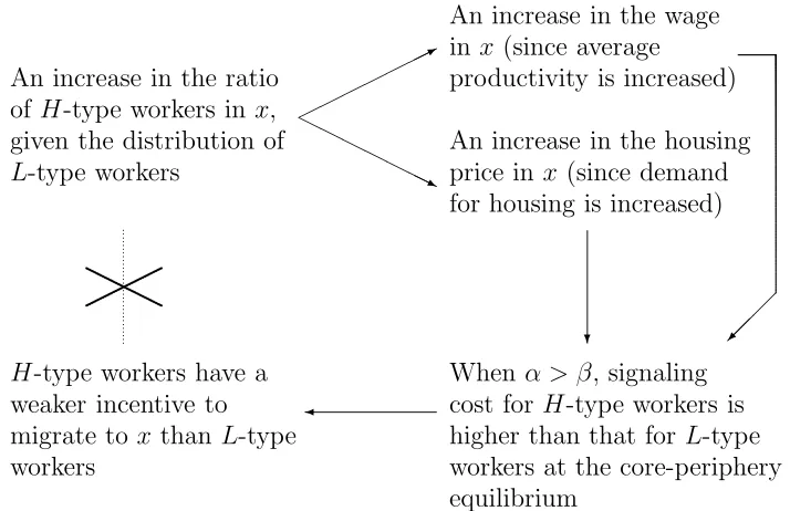
An increase in the ratio of H-type workers in x, given the distribution of
L-type workers
✟✟✟✟ ✟✟✟✯
❍❍ ❍❍
❍❍❍❥
An increase in the wage inx (since average
productivity is increased)
✠
An increase in the housing price in x (since demand for housing is increased)
❄
When α > β, signaling cost for H-type workers is higher than that forL-type workers at the core-periphery equilibrium
✛ H-type workers have a weaker incentive to migrate to x than L-type workers
[image:29.612.114.471.400.631.2]✲ ✛ ✻ ❄ ✛
✻ ❄
✲ ✻ ❄
✛
❄
✲ ✻
45◦ line
A
B E
˙
ρH = 0 ˙
ρL= 0
0 1
1
ρH
ρL
Figure 4: When α < β, there exist two stable core-periphery equilibria, points A and B. In addition, when φH′(ρH)< 0 at ρH = 1
2, the completely
✛ ✲ ✻ ❄ ✛
✻ ❄
✲ ✻ ❄
✛
❄
✲ ✻
45◦ line
A
B
E
˙
ρH = 0 ˙
ρL= 0
0 1
1
ρH
ρL
Figure 5: When α < β and φH′(ρH) > 0 at ρH = 1
2, there exist stable
✲ ✛ ✻ ❄ ✲
✻ ❄
✛ ✻ ❄
✛
❄
✲ ✻
45◦ line
˙
ρL= 0 ˙
ρH = 0
E
0 1
1
ρH
ρL
Figure 6: When α > β and φH′(ρH) <0 at ρH = 1
2, there exists a unique
✛ ✲ ✻ ❄
✲ ✻ ❄
✛ ✻ ❄
✛
❄
✲ ✻
45◦ line
E
˙
ρL = 0 ˙
ρH = 0
0 1
1
ρH
ρL
Figure 7: When α > β and φH′(ρH) >0 at ρH = 1
2, there exists a unique
YL+α n2
¯
s nL
YL 1
1 2
0 YH
ρH
Figure 8: The core-periphery bifurcation when productivity and the mar-ginal utility of housing are negatively correlated, i.e., α < β.
✲ YL+ α n2
¯
s nL
YL 1
1 2
0
ρH
YH

![Table 1: Source: U.S. Census Bureau [1990], (CPH-2).](https://thumb-us.123doks.com/thumbv2/123dok_us/7869901.738359/28.612.110.488.274.406/table-source-u-s-census-bureau-cph.webp)