Munich Personal RePEc Archive
Demand for Money in the Asian
Countries: A Systems GMM Panel Data
Approach and Structural Breaks
Rao, B. Bhaskara and Tamazian, Artur and Singh, Prakash
University of Western Sydney, University of Santiago de
Compostela, Institute of Economic Growth
5 May 2009
Online at
https://mpra.ub.uni-muenchen.de/15030/
Demand for Money in the Asian Countries:
A Systems GMM Panel Data Approach
and Structural Breaks
B. Bhaskara Rao
raob123@bigpond.com
School of Economics and Finance
University of Western Sydney, Sydney, Australia
Artur Tamazian
artur.tamazian@usc.es
School of Economics and Business Administration
University of Santiago de Compostela, Santiago de Compostela, Spain
Prakash Singh
prakash.archa@gmail.com
Institute of Economic Growth, New Delhi, India
Abstract
A systems GMM method is used to estimate the demand for money (M1) for a panel of 11 Asian
countries from 1970 to 2007. This method has advantages of which the most important one is its
ability to minimise small sample bias with persistence in the variables. This system GMM method
of Blundell and Bond (1998) simultaneously estimates specifications with the levels and first
differences specifications of the variables. We test for structural stability of the estimated function
with a recently developed test, for this approach, by Mancini-Griffoli and Pauwels (2006). Our
results show that there is a well defined demand for money for these countries and there are no
structural breaks.
Keywords: Systems GMM, Blundell and Bond, Mancini-Griffoli and Pauwels, Asian Countries
and Demand for Money and Structural Stability.
1. Introduction
Demand for money and its stability have received much attention in the country specific time
series studies. This has been stimulated further after the worldwide financial reforms. It is now an
almost stylized fact that the demand for narrow and broad money has become temporally unstable
in the developed countries after the financial reforms. Reforms have increased competition in the
financial markets, creation of money substitutes like credit cards, electronic money transfers,
increased liquidity of bank deposits and international capital mobility. Many central banks in the
developed countries have found it is hard to predict demand for money and abandoned money
supply as the policy instrument because it is difficult to formulate money supply targets. At the
same time the Taylor rule has made the use of bank rate more attractive as the monetary policy
instrument by arguing that it will increase negative feedback mechanisms and the economy will
become more stable. Therefore, since the late 1970s, many central banks in the developed
countries have switched over from targeting money supply to the rate of interest as the monetary
policy instrument. This is also consistent with Poole (1970) who showed that the rate of interest
should be targeted if the demand for money is unstable.1
Following these developments, central banks in many developing countries have also started using
the rate of interest as their monetary policy instrument without any convincing evidence that their
money demand functions have become unstable. Bahmani-Oskooee and Rehman (2005) found,
with country specific time series methods, that the demand for money functions of several
developing Asian countries are stable.2 According to Poole (1970) if demand for money is stable,
1
Poole’s arguments are well explained in Mishkin (2003) pp.459-463. However, Rao (2007) has argued that central
banks should not be given the power to change the interest rates because such changes have significant distributional
effects. The recent worldwide severe downturn seems to be due to artificially lowering of the interest rate by the FED
in the USA. If interest rates were left to be determined by the market forces, perhaps we could have avoided credit
bubbles, accumulation of huge toxic loans and severe downturns.
2
Countries selected by Bahmani-Oskooee and Rehman are (1) India, (2) Indonesia, (3) Malaysia, (4) Pakistan, (5) the
Philippines, (6) Singapore and (7) Thailand. They found that while in India, Indonesia and Singapore, demand for M1
is stable, in Malaysia, Pakistan, the Philippines and Thailand demand for broader measure (M2) is stable. In these
latter 4 countries the cointegrating equations with M1 are not well determined. However, in a recent paper Sumner
(2008), with data from 1950 to 1998, showed that the components of the demand for money (M1 and M2) in Thailand
have been stable. In our paper we shall use M1 for analysis because M1 is by and large the dominant component of
money supply in the developing countries. In particular it is hard to control NBFI in the organized and unorganized
central banks should use money supply as the monetary policy instrument. Using the rate of
interest as the policy instrument will only accentuate instability.3 Therefore, it is important to
know if the money demand functions in the developing countries have also become unstable.
Stable money demand implies that using the rate of interest as the monetary policy instrument
leads to more instability in the economy. The recent worldwide downturn also raises serious
doubts on using the interest rate as monetary policy instrument even in the developed countries. It
is likely that financial reforms have had their major effects by now implying that the demand for
money may have become more stable since the mid 2000s. However, this conjecture needs further
investigation.4
The objectives of the current paper are twofold. First, we estimate the demand for money with
panel data from 11 Asian countries for the period 1970 to 2007. We shall use a systems based
General Method of Moments (GMM) of Blundell and Bond (1998) for estimation. This has several
advantages. Perhaps our paper is the first to use this method to estimate demand for money with
panel data. Second, we will examine if there has been instability in this relationship after the
financial reforms because this has implications for the choice of monetary policy instruments.5
While many East Asian countries have liberalized financial markets from the early 1980s, the
South Asian countries were late starters and delayed reforms until the early 1990s. Furthermore,
reforms seem to have been introduced without considering the adequacy of the existing banking
and regulatory laws. Consequently, the East Asian countries had a major financial crisis during
1997-1998. In countries like India several non banking financial intermediaries, known as
chit-funds, were established. They have mobilized large amounts of deposits by offering higher interest
rates but many became insolvent due to the week regulatory laws and inadequacies in enforcement
agencies in the Indian banking sector. Therefore, while analysing the temporal stability in the
demand for money, due to financial reforms, a single break date might be somewhat restrictive.
With these perspectives, the outline of this paper is as follows. Section 2 discusses the merits of
the systems GMM. Section 3 presents empirical results. In Section 4 a recent method developed by
using M2 or M3 as alternative measures but perhaps Sumner’s approach is more useful and our methodology can be
also used for different measures of money.
3
Poole’s results are based on the instability in the IS and LM relations. However, instability in the demand for money
is the major cause of instability in LM.
4
In a separate paper we will be using the approach in this paper to analyze demand for money in the OECD countries.
5
Rao and Kumar (2009) have estimated demand for money with a panel of 14 Asian countries with time series
Mancini-Griffoli and Pauwels (2006) for structural stability is discussed and used. Finally Section
5 concludes.
2. Systems GMM Estimates
Generalised Method of Moment (GMM) proposed by Arellano and Bond (1991) is the commonly
employed estimation procedure to estimate the parameters in a dynamic panel data model. In
GMM based estimation, first differenced transformed series are used to adjust the unobserved
individual specific heterogeneity in the series. But Blundell and Bond (1998) found that this has
poor finite sample properties in terms of bias and precision, when the series are persistent and the
instruments are weak predictors of the endogenous changes. Arellano and Bover (1995) and
Blundell and Bond (1998) proposed a systems based approach to overcome these limitations in the
dynamic panel data. This method uses extra moment conditions that rely on certain stationarity
conditions of the initial observation.
The systems GMM estimator thus combines the standard set of equations in first differences with
suitably lagged levels as instruments, with an additional set of equations in the levels with lagged
first differences as instruments. Although the levels of Yit are necessarily correlated with the
individual-specific effects (ηi) given model (1) below, assuming that the first-differences ∆Yitare
not correlated with ηi, and thus permitting lagged first-differences to be used as instruments in the
levels equations.
, 1 1 (1)
it i t i it
Y =αY − + +η ν α <
Results of the Monte Carlo simulation show that the system based GMM approach has better finite
sample properties in terms of bias and root mean squared error than that of GMM estimator with
first differences alone. It is argued by Blundell and Bond (1998) that the systems GMM estimator
performs better than the simple GMM estimator because the instruments in the levels equation
remain good predictors for the endogenous variables in this model even when the series are very
persistent. Though it is argued that system based GMM approach uses more instruments than the
standard GMM and many instruments problem could be serious, in the simulation results this is not
found to be a limitation. In fact simulation results show that the systems GMM estimates are less
3. Empirical Results
With this backdrop we present in Table 1 parameter estimates with alternative specifications of the
demand for money with the standard and systems GMM methods. The standard specification,
based on the quantity theory of money, used in many empirical works in several country specific
time series models, ignoring the error term, is:
0 1 2
1 2
ln ln (2)
1and 0
d
t t t
m α α y α R
α α
= + +
≈ <
where m=real narrow money, y=real output, R=nominal rate of interest, usually measured as
the rate on 3 to 6 month bills and used as a proxy for the opportunity cost of holding money
instead of less liquid assets such as time deposits. Sometimes additional variables are added to (2)
as better proxies for the opportunity cost, especially when the bank rate is set by the central banks
and kept below the market rate. This is generally true in many developing countries and
consequently interest rate in general shows only small variations. For this reason,
Bahmani-Oskooee and Rehman (2005), have ignored R and proxied the opportunity cost with the rate of
inflation (π) and the exchange rate (EX ). EX is measured as the number local currency units for
a unit of foreign currency implying that an increase in EX is devaluation.6 The Bahmani-Oskooee
and Rehman specification, for the Asian countries is:
0 1 3 4
3 4
ln ln ln (3)
0; 0 d
t t t t
m α α y α EX α π
α α
= + + +
< <
Their justification for including EX is that there is currency substitution. However, opportunities
for holding foreign currencies are generally limited in the developing countries, but it is likely that
EX or its rate of change is used as a proxy by households and firms for the expected rate of
inflation and a rise in the real cost of holding money. Therefore, any devaluation of currency will
6
In the money demand for India Rao and Singh (2005) have added a time trend but this was dropped later because its
coefficient was insignificant. They found that the rate of interest was significant but did not use the Bahmani-Oskooee
and Rehman variables inflation rate and exchange rate. With a similar specification Chien-Chiang Lee and Mei-Se
Chien (2008) have also found that the coefficient of the rate of interest is significant in the demand functions for
narrow and broad money for China. They have found that demand for broad money (M2) might have undergone
reduce the demand for money. We shall use the following specification by adding to the standard
specification as in the equation (2) the two additional variables of Bahmani-Oskooee and Rehman
and let the data determine which variables are significant and measure the cost of holding money
better. Further, instead of the level of the interest rate we shall use its logarithm to readily capture
its elasticity.
0 1 2 3 4
ln ln ln ln ln (4)
d
t t t t t
m =α α+ y +α R +α EX +α π
It is likely that R EX, and π and/or their rates of change (if these variables have temporary
dynamic effects) are used by money holders with different weights as proxies to form expectations
about the opportunity cost of holding liquid money.
Our panel sample is for the period 1970 to 2007 with 11 Asian countries. These are Bangladesh,
China, Hong Kong, India, Indonesia, Korea, Malaysia, the Philippines, Singapore, Sri Lanka and
Thailand. Originally we have included Pakistan, but due to lack of adequate data on the rate of
interest it was dropped. Detail of the data sources and definitions of the variables are in the
appendix.
We have used first the standard panel data methods to estimate equation (2) with OLS with the 11
means of the variables. This is also known as TOTAL estimates. Next, we estimated the fixed
effects (BETWEEN and WITHIN) and the random effects (REF) models. The REF model is
estimated with the Generalised Least Squares (GLS). The estimates with these four methods are in
Table 1 Conventional Panel Data Estimates of Demand for Money 1972-2007
0 1 2 3 4
ln d ln ln ln ln
t t t t t
m =α α+ y +α R +α EX +α π
1 2 3 4 5 6 7 8
TOTAL BETWEEN WITHIN REM TOTAL BETWEEN WITHIN REM
1
α
0.361 [0.00] 0.228 [0.26] 1.188 [0.00] 1.169 [0.00] 1.363 [0.00] 0.941 [0.00] 1.975 [0.00] 1.982 [0.00] 2α
-1.197 [0.00] -1.745 [0.22] 0.137 [0.07] 0.109 [0.14] -- -- -- -- 3α
-- -- -- -- -1.456[0.00] -0.873 [0.03] -1.686 [0.00] -1.727 [0.00] 4
α
-- -- -- -- -3.925[0.00] -20.117 [0.13] -0.507 [0.07] -0.580 [0.03] 0
α
-2.211 [0.00] -2.406 [0.53] -5.454[0.00] -2.192 [0.00] 0.262 [0.83] -- -6.220 [0.00] ___ 2
R 0.288 0.220 0.914 0.177 0.782 0.812 0.965 0.666
DW 0.027
[0.00]
-- 0.169
[0.00]
0.669E-2 [0.00]
0.133 [0.00]
-- 0.231 [0.00]
0.013 [0.00]
It can be observed from the first 4 columns that the results are mixed and the DW statistics is
significant, indicating the presence of serial correlation in the residuals. Hence, we reestimated this
equation while allowing for first order serial correlation in the REM but the likelihood function did
not converge which confirms that these variables are highly persistent. This conjecture is plausible
because many time series studies have found that income and money etc., are I(1) in levels.
Subject to these caveats and the fact that the computed standard errors are unreliable and probably
underestimated, we can say that only estimates of WITHIN and REM in columns 3 and 4, where
the income elasticity is close to unity, as found in many country specific time series studies, seem
to be reasonably acceptable. Both WITHIN and REM estimates indicate that the coefficient of the
rate of interest has wrong sign and insignificant at the 5% level.
Consequently, we have dropped the rate of interest and estimated the Bahmani-Oskooee and
Rehman specification of equation (3). These results are reported in columns (5) to (8) of Table 1.
Though these results have improved significantly with much higher adjusted R s2 , the significant
DW statistics show that serial correlation still persists. Our attempt to reestimate the serial
correlation coefficient with the REM met the same convergence problems. It is somewhat
8) estimates far exceed the stylised value of unity. The main conclusions that can be drawn from
the conventional panel data estimates are as follows. First, the estimates are sensitive to the
method of estimation and specification. Second, if the variables are non-stationary, it is difficult to
minimise the serial correlation in the residuals. Finally, perhaps the rate of interest is not a good
indicator of the opportunity cost of liquidity compared to the Bahmani-Oskooee and Rehman’s
preference for the exchange rate and inflation rate.
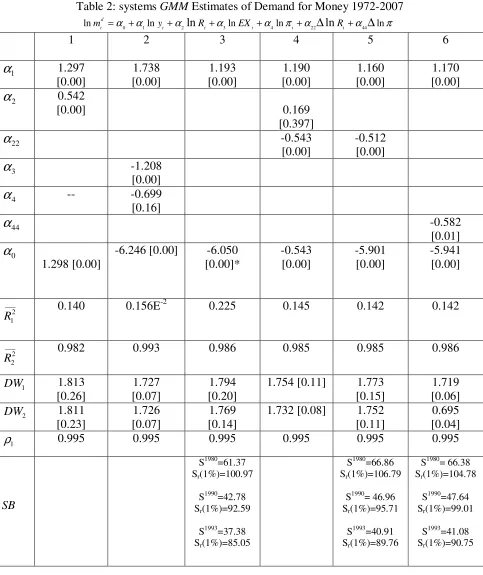
With this hindsight, we now estimate the basic equation (2) with the systems GMM. Results are in
column 1 of Table 2. Since estimates with the conventional methods indicated that there is serial
correlation, we estimated the first order serial correlationρ1and found that it is almost unity
indicating that persistence in the variables is very high. Therefore, these estimates are made by
transforming the levels equation for first order serial correlation with the assumption that
1 0.995
ρ = to achieve convergence. These estimates of equation (2) are far superior to those in
Table 1, but the coefficient of the rate of interest has the wrong sign. The null that the coefficient
of income is unity could not be rejected by the Wald test. The computed test statistics with the
p-value in the square brackets is χ12 =2.624[0.11].
As before, we omitted the rate of interest and then estimated the Bahmani-Oskooee and Rehman
specification in (3) and the results are reported in column 2 of Table 2. This equation is also better
determined than the equation in Table 1. The adjusted R2for the levels equation, denoted as __
2 2,
R is
very high and DW2 for this equation shows that there is no further first order serial correlation.
Although the 3 coefficients have the expected sings, the coefficient of the rate of inflation is
insignificant and that of income well exceeds unity. This is also the case with the estimates based
on WITHIN (column 7) and REM (column 8) in Table 1.
We have deleted all the opportunity cost variables and estimated the demand for money only as a
function of income. These results are presented in column (3) of Table 2 and they gave a better
result. The adjusted R2of the levels and differences equations have increased and the DW
statistics of both equations show that there is no serial correlation. The estimated income elasticity
To further improve these estimates, we added changes in the rate of interest as an additional
variable. This can be justified because central banks do not change the bank rate on a daily basis
or frequently. Therefore, money holders and media take notice of changes in the rate of interest
instead of its level. Such changes may have some effects in the short run. The same justification
[image:10.595.69.552.73.648.2]applies to the changes in the exchange rate and the rate of inflation. Estimates with the change in Table 2: systems GMM Estimates of Demand for Money 1972-2007
0 1 2 3 4 22 44
ln d ln ln ln ln ln ln
t t t t t t
m =α α+ y +α R +α EX +α π α+ ∆ R +α ∆ π
1 2 3 4 5 6
1
α
1.297 [0.00] 1.738 [0.00] 1.193 [0.00] 1.190 [0.00] 1.160 [0.00] 1.170 [0.00] 2α
0.542[0.00] 0.169
[0.397] 22
α
-0.543 [0.00] -0.512 [0.00] 3α
-1.208 [0.00] 4α
-- -0.699[0.16] 44
α
-0.582 [0.01] 0α
1.298 [0.00]-6.246 [0.00] -6.050 [0.00]* -0.543 [0.00] -5.901 [0.00] -5.941 [0.00] ___ 2 1
R 0.140 0.156E
-2
0.225 0.145 0.142 0.142
___ 2 2
R 0.982 0.993 0.986 0.985 0.985 0.986
1 DW 1.813 [0.26] 1.727 [0.07] 1.794 [0.20]
1.754 [0.11] 1.773 [0.15] 1.719 [0.06] 2 DW 1.811 [0.23] 1.726 [0.07] 1.769 [0.14]
1.732 [0.08] 1.752 [0.11]
0.695 [0.04]
1
ρ 0.995 0.995 0.995 0.995 0.995 0.995
SB
S1980=61.37 Sr(1%)=100.97
S1990=42.78 Sr(1%)=92.59
S1993=37.38 Sr(1%)=85.05
S1980=66.86 Sr(1%)=106.79
S1990= 46.96 Sr(1%)=95.71
S1993=40.91 Sr(1%)=89.76
S1980= 66.38 Sr(1%)=104.78
S1990=47.64 Sr(1%)=99.01
the rate of interest are in column (4). As can be noticed the change in the rate of interest has the
correct negative sign and significant. There is no significant change in the estimate of income
elasticity. The Wald test static χ12 =0.504[0.48]could not reject the null that income elasticity is
unity. We have added changes in the exchange rate and the rate of acceleration in the inflation rate
as additional variables but found that the coefficient of changes in the exchange and interest rates
became insignificant. Income elasticity remained close to unity. We then estimated various
combinations of these variables and found that one another of these variables became insignificant.
To conserve space these results are not reported. Finally, we estimated by replacing the change in
the rate of interest with the rate of acceleration in inflation. This estimate is reported in column (5)
and it is as good as the estimate in column (4). A noteworthy feature of all these alternative
estimates is that income elasticity has remained near unity. Therefore, the specifications
underlying the estimates in columns (4) and (5) are more robust than all other alternatives.
Estimates in column (4) are marginally preferable because its DW statistic for the levels equation
rejects serial correlation in the residuals more conclusively. Nevertheless, we shall subject these
two equations for structural break tests.
4. Structural Breaks
At the outset it may be noted that if there are structural breaks, it does not imply that money
demand has become unstable. It is likely that money demand if estimated for the period before and
after the breaks may be well behaved except that some parameters may show small or significant
changes. For money demand to become unstable and useless for predictions and policy use, its
estimates after the break dates should indicate large standard errors and implausible estimates of
the parameters. We now intend to test for structural breaks in the equations in columns (4) and (5)
for their different break dates. While many studies on money demand functions for the Asian
countries with country specific time series data found no major structural breaks, as far as we are
aware only Chien-Chiang Lee and Mei-Se Chien (2009) have found in their interesting study that
there are structural breaks in the demand for money for China in 1980 and 1993. It is difficult to
accept these dates as common break dates for all the countries in our panel because, first, reforms
have been implemented at different dates by different countries. Second, due to lack of effective
regulatory mechanisms, these reforms may have had different effects at different dates. Finally,
there do not seem to be structural break tests for panel data estimates with classical methods where
the break dates are endogenously determined. Because of these limitations, we have selected 1990
as the break date partly, as this would give about the same number of time series observations
financial crisis of 1997-1998. Nevertheless, we will also consider 1980 as a possible break date
and 1990 is close to 1993 of Chien-Chiang Lee and Mei-Se Chien.
It would be useful if we understand first the nature of the recently developed structural break tests
for the dynamic panel data models. We have used Mancini-Grifoli and Pauwels (2006) procedure
to detect possible structural breaks. This new procedure offers three main practical and technical
advantages over others. First, the test does not make any distributional assumptions as it estimates
empirically the distribution of the test statistic using an empirical sub-sampling methodology.
Second, the power of the test remains high even there are very few observations after the break
date. Third, the test requires very few regularity conditions. It remains asymptotically valid despite
non-normal, heteroscedastic and/or autocorrelated errors, and non-strictly exogenous regressors.
Here we wish to highlight that among other tests, an important advantage of this one is that it does
not require normal iid errors and strictly exogenous regressors, while the F-type tests do impose
these restrictions.Hence, the regression that serves as the basis for test of structural break has the
following general form:
0 1 1,..., (5) 1,..., it it it
it t it
X U t T
Y
X U t T T m
β β ′ + = = ′ + = + +
for individuals i=1,...,n and where T is the supposed break date. The test hinges the next
hypotheses: H0 :β1t =β0 againstHA :β1t ≠β0. In order to build the test, Mancini-Grifoli and
Pauwels consider more observations after the break date than regressorsd , (m×n)≥d. Briefly,
the test statistic is a positive definite quadratic form obtained from the transformed (m×n)≥1
vector of residuals by the (m×n)×(m×n) covariance matrix, projected onto the column space of
d n m× )×
( matrix of transformed post-instability regressors. As the authors argue, the equivalent
of the generic test statistic in Andrews (2003) for panel data can be defined after considering an
interval τr which goes from
[
r,r+m−1]
and where r∈{
1,...,T +1}
, as:(
)
(
)
(
)
(
)
( )
1 1 1, , , , (6)
ˆ ˆ
, , (7)
ˆ (8)
r r r r
r r T m r
r r T m r
S A V A
A X W
V X X
τ τ
τ τ
β
β
β
with τ
(
τ τβ
)
r r r
Wˆ = Υ −Χ where r
Wˆ is the τ (m×n)×1 residual vector of observations starting at
r, with β =βˆT+m defined to be the coefficient vector estimated over the T +m. The
variance-covariance matrix, ΣˆT+m, is given by:
(
)
1 1(
)
1
ˆ 1 T ˆ ˆ (9)
T m r r
r
T U Uτ τ
+ − +
=
′ ∑ = +
∑
where the
(
m×n)
×1 residual vector, Uˆ , is defined as τr(
T m)
r r r
Uˆτ = Υτ −Χτ βˆ + . It is noteworthy that this covariance matrix corrects for serially correlated errors, heteroscedasticity and potential
cross-sectional correlation.
The particular form of the test statistic for the post-break residuals is defined as:
(
)
1 ˆ , ˆ (10)
T T m T m
S =S + β + ∑ +
At the same time, the critical values,Sr, are found by empirically generating a distribution
function for the statistic under the null of stability. As before, if
(
m×n)
≥d the T −m+1 differentr
S values are defined as:
(
ˆ ,2 ( ), ˆ)
(11)r r r T m
S =S β ∑ +
whereβˆ2,(r) is the estimate of β over t =1,...,Tobservations but excluding
2
m
observations. The
optimization of the power and size is the reason behind such exclusion, compared with the
exclusion of only m observations or no observations at all.
As it can be observed from the last row of Table 2, the computed test statistics are less than the
critical values at the 1% level. Therefore, we could not confirm the existence of structural breaks
in 1980, 1990 nor 1993. It may be concluded that demand for money has been stable for the panel
of our Asian countries and money supply should be used by their central banks as the monetary
5. Conclusions
In this paper we have used the standard and Bahmani-Oskooee and Rehman (2005) specifications
plus a modified specification with the changes in the rate of interest and inflation rate to estimate
the demand for money with traditional panel OLS, two panel fixed effects and panel random effect
(REM) techniques. Results of these estimates suffer from the problem of serial correlation in the
residuals. Even after allowing for the first order serial correlation the REM estimates show
persistence in the variables. In the light of conventional panel data estimation, it can be said that
parameter estimates are sensitive to method of estimation and also to the specification of the
model. Again, if the variables are non stationary conventional methods do not help estimation and
can provide less reliable results. Estimates with the System GMM seems to go a long way to
minimise persistence problem. These systems based estimates show that the income elasticity of
the demand for money is unity and rate of interest is not the best indicator of the opportunity cost
holding money (liquidity). The change in the rate of interest and the rate of acceleration of
inflation are found to be better proxies for the cost of holding money than the level of interest rate
and the rate of inflation.
Result with the Mancini-Grifoli and Pauwels (2006) structural break test on the stability of the
demand for money showed that demand for money in these 11 Asian countries does not suffer
from structural breaks due to financial reforms. This may be due to a possibility that financial
reforms are yet to have significant effects in increasing money substitutes, electronic transfers and
increase the competitiveness in the financial markets. hus it can be argued that demand for money
functions in these countries are stable. Therefore, money supply should be used as the monetary
policy instrument by their central banks as explained by Poole (1970).
Even though our results are fairly robust and imply a stable demand for money in the panel of the
11 Asian countries, it has some limitations. Initially we had a panel of 12 countries for the study
but due to lack of sufficient number of observation for Pakistan, we dropped it from the
estimation. It is desirable to increase the cross section dimension in future studies. Our selection of
the break dates is not endogenous, but given the fact that we do not have better and satisfactory
methods to decide endogenously the break dates in the panel data, we had to be pragmatic in our
choice of techniques. In spite of these limitations we hope that our paper will provide incentives
References
Arellano, M. and Bond, S.R. (1991). Some tests of specification for panel data: Monte Carlo
evidence and an application to employment equations, Review of Economic Studies, 58, 277-297.
Arellano, M. and Bover, O. (1995). Another look am the instrumental variable estimation of
error-component models, Journal of Econometrics, 68, 29-45.
Bahmani-Oskooee, M. and Rehman, H. (2005). Stability of the money demand function in 651
Asian developing countries. Applied Economics, 37, 773–792.
Blundell, R. and Bond, S. (1998). Initial conditions and moment restrictions in dynamic panel data
models, Journal of Econometrics, 87, 115-43.
Lee, C. C. and Chien, M-S. (2008). Stability of money demand function revisited in China,
Applied Economics, 40, 3185-3197.
Mancini-Griffoli, T. and Pauwels, L. L. (2006). Is There a Euro Effect on Trade? An Application
of End-of-Sample Structural Break Tests for Panel Data, HEI Working Papers 04-2006.
Mishkin, F.S. (2003). The Economics of Money, Banking and Financial Markets, 6th ed. 679
Addison and Wesley, New York.
Poole, W. (1970). The optimal choice of monetary policy instruments in a simple macro 696
model. Quarterly Journal of Economics 84: 192–216.
Rao, B. B. and Singh, R. (2005). Demand for money in India: 1953-2003, Applied Economics, 38:
1319–1326.
Rao, B. B. (2007). The nature of the ADAS model based on the ISLM model, Cambridge Journal
of Economics, 31: 413-422.
Rao, B.B, and Kumar, S. (2009). A Panel data approach to the demand for money and the effects