http://dx.doi.org/10.4236/cn.2013.54034
Genetic Algorithm Based Node Deployment in Hybrid
Wireless Sensor Networks
Omar Banimelhem1, Moad Mowafi1, Walid Aljoby2
1Department of Network Engineering and Security, Jordan University of Science and Technology, Irbid, Jordan 2Department of Computer Engineering, Jordan University of Science and Technology, Irbid, Jordan
Email: [email protected], [email protected], [email protected]
Received July 4, 2013; revised August 1, 2013; accepted August 8, 2013
Copyright © 2013 Omar Banimelhem et al. This is an open access article distributed under the Creative Commons Attribution Li- cense, which permits unrestricted use, distribution, and reproduction in any medium, provided the original work is properly cited.
ABSTRACT
In hybrid wireless sensor networks composed of both static and mobile sensor nodes, the random deployment of sta- tionary nodes may cause coverage holes in the sensing field. Hence, mobile sensor nodes are added after the initial de- ployment to overcome the coverage holes problem. To achieve optimal coverage, an efficient algorithm should be em- ployed to find the best positions of the additional mobile nodes. This paper presents a genetic algorithm that searches for an optimal or near optimal solution to the coverage holes problem. The proposed algorithm determines the minimum number and the best locations of the mobile nodes that need to be added after the initial deployment of the stationary nodes. The performance of the genetic algorithm was evaluated using several metrics, and the simulation results dem- onstrated that the proposed algorithm can optimize the network coverage in terms of the overall coverage ratio and the number of additional mobile nodes.
Keywords: Target Coverage; Node Deployment; Genetic Algorithm; Wireless Sensor Networks
1. Introduction
A Wireless Sensor Network (WSN) is a distributed sys- tem which is composed of tiny, low-cost, battery-oper- ated sensor nodes that collaborate together for the pur- pose of achieving certain task such as environment moni- toring and object tracking [1]. Depending on the required application, the sensor nodes are responsible for sensing, computation and communication tasks. The sensing task is usually configured in each node; therefore the sensing attribute is considered a key factor in designing WSNs.
One of the key points in the design stage of a WSN that is related to the sensing attribute is the coverage of the sensing field. In the literature, the coverage problem in WSNs has been addressed either as target coverage or area coverage [2]. While area coverage protocols are designed to maximize the area of the sensing field that could be covered, target coverage, on the other hand, assumes that the sensing field is divided into targets. Therefore, the main objective of the target coverage pro- tocols is to maximize the number of targets that could be covered in the field.
The coverage issue in WSNs depends on many factors, such as the network topology, sensor sensing model, and
the most important one is the deployment strategy that is used to distribute or throw the sensor nodes in the field [3]. The sensor nodes can be deployed either manually based on a pre-defined design of the sensor locations, or randomly by dropping them from an aircraft. Random deployment is usually preferred in large scale WSNs not only because it is easy and less expensive but also be- cause it might be the only choice in remote and hostile environments. However, random deployment of the sen- sor nodes can cause holes formulation; therefore, in most cases, random deployment is not guaranteed to be effi- cient for achieving the required objective in terms of the coverage [2].
man intervention is not possible or when the sensing filed is hostile, random deployment is the only choice.
In random deployment, the holes formulation problem might be reduced or eliminated after initial deployment using one of two approaches. In the first approach, if all sensor nodes are mobile, then an efficient algorithm should be designed such that the coverage is maximized while at the same time the moving cost of the mobile nodes is minimized. In this case, the mobility feature of the nodes can be utilized in order to maximize the cov- erage. After the initial configuration of the mobile nodes in the sensing field, an efficient algorithm such as poten- tial field algorithm or virtual force algorithm can be em- ployed for the purpose of relocating the sensor nodes [4,5].
In the second approach, if the sensor nodes are hybrid in which some of the nodes are stationary and the other are mobile, an efficient algorithm should be employed in order to find the number and locations of the mobile nodes that should be added after the initial deployment of the stationary nodes. One of the algorithms that can be employed is a genetic algorithm (GA) which is used to find an optimal or near optimal solution for optimization problems [6]. A little research in the field of WSNs has used and employed GA to search for an optimal number of sensor nodes that can be added after the initial node deployment in order to maximize the coverage.
In this paper, we propose an approach that exploits the movements of some nodes for eliminating the holes which would be formulated after the initial deployment of the sensor nodes. Our approach uses GA in order to determine the minimum number of mobile nodes that should be used in addition to the previously deployed stationary nodes such that the coverage of the monitored area is maximized.
This paper is organized as follows. Section 2 discusses the operation of the GA. Section 3 presents the related work. Section 4 discusses the assumptions and the com- ponents of the proposed approach. Section 5 presents simulation experiments and discusses the results, and Section 6 concludes the paper.
2. Genetic Algorithm
A genetic algorithm is used to search for near optimal solutions when no deterministic method exists or if the deterministic method is computationally complex. GA is a population based algorithm (i.e.; it generates multiple
solutions each iteration). The number of solutions per iteration is called population size. Each solution is repre- sented as a chromosome and each chromosome is built up from genes. For a genetic algorithm of population size
n, it starts with n random solutions. Then it chooses the
best member solutions for mating to generate new solu- tions. The best generated solutions will be added to the
next iteration while the bad solutions will be rejected. While the algorithm iterates its solutions, these solutions are improved up to a point where converge to a near op- timal solution is achieved. Many factors should be taken into consideration when the genetic algorithm is used. The first factor is the representation of chromosome and genes because bad representation may result in slower convergence. Another important factor is the mechanism of producing new solutions from the old ones. The most popular mechanisms are crossover and mutation. The third factor is how to find a fitness function (i.e.; a me-
thod to evaluate the solutions) in order to accept or reject the solutions, and how to select the best members for mating.
In general, a genetic algorithm has four stages: popu- lation initialization, evaluation of fitness, reproduction and termination. Initialization is the process of creating initial random solutions, which can be done by setting genes to random values. In the initialization process, n
chromosomes are created as the first generation of solu- tions. After the initialization, each chromosome fitness (i.e.; solution goodness) is evaluated using the fitness
function.
Reproduction process has four steps: selection, cross- over, mutation, and accepting the solution. In the selec- tion step, the fittest members in the current population are selected in order to reproduce new solutions. How- ever, less fitness members will have also a chance to be selected. The selection step can be implemented by many mechanisms such as the rollet wheel method. This selec- tion will be performed on two chromosomes to reproduce two new chromosomes each time. After selecting the chromosomes, a crossover operation is performed by selecting a random point in chromosomes and exchang- ing genes after this point. Crossover may be stuck in lo- cal optima. To overcome this problem, a tie breaker is needed which can be achieved by using mutation opera- tion where a gene is selected randomly and its value is changed.
A widely used representation for genes is bits where each gene is represented by a bit. In this case, mutation is done by flipping a bit randomly in the chromosome. Af- ter crossover and mutation, two new chromosomes are reproduced. The final step is accepting these two chro- mosomes to be in the new population. Typically, the new chromosomes are accepted if they are better than their parents.
3. Related Work
Several research works have addressed the node deploy- ment problem to achieve maximum coverage in WSN. For random node deployment, these works considered WSNs that consist of mobile sensor nodes [4,5,7,8] or that contain both static and mobile nodes [9-12].
For mobile sensor networks, several approaches have been proposed. Voronoi diagrams were used in [7] to find the uncovered areas and determine the positions where the nodes can move. In [4], a potential field-based approach was proposed, in which a repelled force is gen- erated between the obstacles and sensor nodes and among the nodes themselves, in order to evenly distribute the nodes in the field. A virtual force algorithm was pro- posed in [5] that uses both pulling and pushing force among the nodes. In [8], simulated annealing was used to find near optimal solutions for nodes placement that maximize the coverage of the area of interest.
On the other hand, several works have considered both static and mobile nodes in WSN. In [9], a bidding proto- col was proposed, in which the static nodes are utilized as bidders and a number of mobile nodes move accord- ingly to satisfy the coverage requirements. In [10], a dis- tributed protocol was proposed that considers the differ- ent sensing capabilities of the nodes using realistic sens- ing coverage model. In this protocol, the static nodes determine the uncovered areas using a probabilistic cov- erage algorithm and the mobile nodes move accordingly using virtual force algorithm. In [11], several approaches were proposed based on virtual force algorithm and par- ticle swarm optimization. The obtained solutions were analyzed for better deployment in the region of interest. Recently, a biogeography-based optimization algorithm was proposed in [12] to maximize the coverage area of the network.
Genetic algorithms have also been used to solve the problem of optimal node deployment. While most of the proposed solutions have focused on deterministic node deployment [13-18], few works have been done in case of random node deployment [19-22]. In random deploy- ment, genetic algorithms are applied to determine near optimal positions for additional mobile nodes in order to maximize the coverage. In [19], a force-based genetic algorithm was proposed, in which the mobile nodes util- ize the sum of the forces used by the neighbors to choose their direction. In [20], a multi-objective genetic algo- rithm running on a base station was used. The base sta- tion determines where the mobile nodes can move to maximize the coverage and minimize the travelled dis- tance. In [21], a cluster based WSN was considered and a genetic algorithm was used to find the best positions for the cluster heads that cover the maximum number of nodes and hence maximizing the area coverage. In [22], Voronoi diagrams were used to partition the field into
cells and a genetic algorithm was then applied to deter- mine the best positions for k additional mobile nodes that maximize the area coverage inside each cell.
Unlike the above-mentioned genetic algorithms, this paper proposes a genetic algorithm that finds the mini- mum number of additional mobile nodes and the best positions for these nodes in order to maximize the overall coverage
4. Proposed Approach
In this section, we present our proposed approach. We first present the network assumptions and coverage model, and then we discuss the GA-based approach.
4.1. Network Assumptions
It was assumed that the sensor nodes are randomly de- ployed and equipped with GPS, and the base station node position is stationary. Furthermore, the number of sensor nodes that are initially deployed equals the number of nodes that are required to achieve full coverage as if these nodes were deterministically deployed. It was also assumed that few mobile nodes are available and can be used to repair the coverage holes after initial deployment of the stationary nodes.
4.2. Coverage Model
We assumed that each sensor node with a sensing radius
r can cover an area of circular shape. We also assumed
that a target object Oj can be detected by sensor Si if Oj is
within the sensing range of Si. This can be represented
using the binary model of sensor detection which is given by:
1, , Coverage
0, , i j
i j
D S O r
S
D S O r
(1)
where D is the distance between the target object being
sensed Oj and the sensor node Si. The coverage function
Coverage(S)equals 1 when the target object can be cov-
ered or sensed, otherwise it equals 0.
4.3. GA-Based Approach
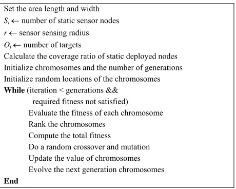
The main objective of employing the GA in our approach is to maximize the coverage by reducing or eliminating the holes that are formulated after initial deployment of the stationary nodes. Figure 1 shows the pseudo code of
the proposed GA algorithm. Assume that Si stationary
sensor nodes are deployed randomly over a sensing field, and all the sensor nodes have the same sensing range which is represented as a circle with radius r. Then, the
Set the area length and width
Si number of static sensor nodes r sensor sensing radius
Oj number of targets
Calculate the coverage ratio of static deployed nodes Initialize chromosomes and the number of generations Initialize random locations of the chromosomes
While (iteration < generations &&
required fitness not satisfied)
Evaluate the fitness of each chromosome Rank the chromosomes
Compute the total fitness
Do a random crossover and mutation Update the value of chromosomes Evolve the next generation chromosomes
[image:4.595.59.289.82.266.2]End
Figure 1. Implementation procedure of the GA-based opti- mization model.
number and locations of the mobile nodes as follow: 1) Chromosmes modeling: Each chromosome, as a
solution in the GA, represents the location of a potential mobile sensor node in the sensing field modeled as (X, Y) point. The gens of each chromosome represent a binary digit that resembles the value of the location on the X and Y axises. For example, in order to represent a mobile node mapped to location (30,40), the corresponding chro- mosome is shown in Figure 2.
The size of the chromosome population is selected based on two factors: the area of the sensing field and the initial configuration of the network. For instance, if the area of the sensing field is 50 m 50 m, the sensing radius of each node is 8m, and the number of deployed stationary nodes is 13 (i.e.; 502/(82) ≈ 13), then the
proposed GA will start with population of 13 randomly generated chromosomes.Note that value 13 is selected in this case based on the assumption that 13 sensor nodes would cover the entire field as if they were determini- stically deployed.
2) Fitness function: In GAs, an objective function is
defined in order to evaluate the fitness of each solution to the corresponding objective. The formulation of the ob- jective or fitness depends on the problem characteristics. The fitness function is used in order to choose the best fittest chromosomes for the purpose of reproduction of the next generated solutions by the GA. The fitness func- tion in our model defines the mutually exclusive cover- age ratio of each chromosome. That is, the fitness func- tion calculates the maximum number of covered targets by each mobile node if and only if these targets are un- covered by other mobile or static nodes. This property of the fitness function prevents the overlapping redundancy among the coverage regions of the deployed mobile nodes and forces each mobile node to cover only a dis- tinct region. The fitness function is given by:
X-location Y-location
0 1 1 1 1 0 1 0 1 0 0 0
Figure 2. Chromosome representation of sensor location (30, 40).
/
1, ,
and ,
, Otherwise
Si Si j
Si j C S i
Si
F M D M O
F M O S F M
F M
r
(2)
where F(MSi) is the fitness of mobile node i (MSi) which
calculates the coverage as a function of the targets it cov- ered, given that the target object Oj is not covered by any
stationary node or other mobile nodes. In Equation (2), Sc
is the coverage of initially deployed stationary nodes and
F(MS/i) is the coverage of any mobile node except mobile
node i.
To choose the fittest species for mating in the next generation, we defined a fitness ratio for each mobile node as a function of its coverage and the total number of targets, which is given by:
Fitness Ratio Si % j F M
O
(3)We also defined a function that measures the total cov- erage of the network at each GA generation. This func- tion is defined as an accumulation of the coverage of the static nodes and the generated mobile nodes, and is given by:
1 Accumulated Coverage mC i S
S F M
i
(4)3) GA operators: We used the fitness ratio calculated
tion, with low probability, is applied to toggle the ran- domly selected gene on the chromosomes.
4) Termination condition:We defined the termination
condition of the applied algorithm in terms of the number of generations and coverage ratio perspectives. That is, the algorithm terminates either when the required net- work coverage ratio is reached or when the algorithm reaches the specified number of generations.
5. Performance Evaluation
In this section, the performance of the proposed algo- rithm is evaluated in terms of the amount of coverage (coverage ratio), degree of coverage (k-coverage), and number of additional mobile nodes. Moreover, the effect of the number of randomly deployed static nodes and the sensing ranges on coverage and number of additional mobile nodes were investigated.
Two simulation experiments were conducted for per- formance evaluation. In the simulation environment, it was assumed that the sensor nodes were randomly de- ployed and the targets were uniformly located in a 200 m
200 m sensor field. In the first experiment, the number of deployed static nodes varies from 100 to 200 to cover 625 targets, whereas the sensing ranges of all nodes are fixed to 12 m. In the second experiment, the number of deployed static nodes is fixed to 100, while the sensing ranges vary from 10 m to 20 m. In each experiment, the coverage ratio, k-coverage, and number of additional mobile nodes were measured before and after applying the proposed algorithm.
[image:5.595.312.537.87.215.2]5.1. Effect of Number of Static Nodes
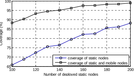
Figure 3 shows the coverage ratio when the static nodes
[image:5.595.311.537.258.387.2] [image:5.595.320.527.428.554.2]are randomly deployed and after adding the mobile nodes to the network. As shown, the coverage ratio increases as the number of deployed static nodes increases. The cov- erage of the static nodes alongside the additional mobile nodes clearly outperforms the case of random deploy- ment of the static nodes as the additional mobile nodes are located into regions where targets are not covered by the static nodes.
Figure 4 shows the k-coverage when the static nodes
are randomly deployed and after adding the mobile nodes to the network. For both cases, it is shown that as the number of nodes increases, the k-coverage increases. This is because the static nodes in both cases are ran- domly deployed and it is very likely that the coverage among these nodes is overlapped, hence the targets would be covered by more sensor nodes as the number of static nodes increases.
Figure 5 shows the number of additional mobile nodes
versus the number of randomly deployed static nodes. As shown, the number of mobile nodes decreases as the
100 120 140 160 180 200
65 70 75 80 85 90 95 100
Number of deployed static nodes
C
ov
er
age (
%
)
coverage of static nodes coverage of static and mobile nodes
Figure 3. Comparison of coverage ratio for different number of deployed nodes.
100 120 140 160 180 200
1.6 1.8 2 2.2 2.4 2.6
Number of deployed static nodes
K
-co
ve
ra
g
e
K-coverage of static nodes K-coverage of static and mobile nodes
Figure 4. Comparison of k-coverage for different number of deployed nodes.
100 120 140 160 180 200
40 45 50 55 60
Number of deployed static nodes
Num
b
er
of
ad
ded m
o
bi
le no
des
mobile nodes vs. static nodes
Figure 5. Number of additional mobile nodes versus number of static nodes.
number of static nodes increases. This is because more targets would be covered as the number of static nodes increases and hence less mobile nodes would be added to increase the coverage ratio.
5.2. Effect of Sensing Range
Figure 6 shows the coverage ratio when the static nodes
sensing range can cover more targets than that with smaller range. The coverage of the static nodes along with the additional mobile nodes clearly outperforms the case of random deployment of the static nodes as the additional mobile nodes are located into regions where targets are not covered by the static nodes.
Figure 7 shows the k-coverage when the static nodes
are randomly deployed and after adding the mobile nodes as a function of the sensing ranges. As shown, the k- coverage increases as the sensing radii of the deployed nodes increase. This is because the coverage among sen- sor nodes with large sensing range is very likely to over- lap, and hence more targets would be covered by multi- ple nodes.
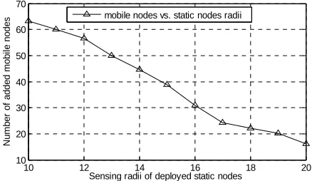
Figure 8 shows the number of additional mobile nodes
as a function of the sensing range. It is shown that the number of mobile nodes decreases as the sensing radii of the nodes increase. This is because more targets would be covered as the sensing range of the static nodes in- creases and hence less mobile nodes would be added to increase the coverage ratio.
6. Conclusion
This paper presents a genetic algorithm to find an opti- mal solution to the coverage holes problem caused by random deployment of stationary sensor nodes in wire-
10 12 14 16 18 20
50 60 70 80 90 100
Sensing radii of deployed static nodes
Cov
e
ra
ge
(
%
)
[image:6.595.62.287.423.554.2]coverage of static nodes coverage of static and mobile nodes
Figure 6. Comparison of coverage ratio for different sensing ranges.
10 12 14 16 18 20
1 1.5 2 2.5 3 3.5
Sensing radii of deployed static nodes
K
-co
ve
ra
g
e
[image:6.595.61.282.593.709.2]K-coverage of static nodes K-coverage of static and mobile nodes
Figure 7. Comparison of k-coverage for different sensing
10 12 14 16 18 20
10 20 30 40 50 60 70
ranges.
Sensing radii of deployed static nodes
N
um
b
er
of
adde
d m
obi
le
nodes
mobile nodes vs. static nodes radii
Figure 8. Number of additional mobile nodes versus sensing
ss sensor networks. The performance of the proposed
[1] I. F. Akyildiz bramaniam and E.
ranges.
le
algorithm was evaluated in terms of the coverage ratio, k-coverage, and the number of additional mobile nodes using different numbers of stationary nodes and various sensing ranges. The simulation results showed that the genetic algorithm can maximize the coverage of the sens- ing field by finding the minimum number of additional mobile nodes and their best positions in the field.
REFERENCES
, W. Su, Y. Sankarasu
Cayirci, “Wireless Sensor Networks: A Survey,” Com- puter Networks, Vol. 38, No. 4, 2002, pp. 393-422.
http://dx.doi.org/10.1016/S1389-1286(01)00302-4 [2] B. Wang, “Coverage Problems in Sensor Networks: A
Survey,” ACM Computing Surveys, Vol. 43, No. 4, 2011,
53 p. http://dx.doi.org/10.1145/1978802.1978811
[3] M. Younis and K. Akkaya, “Strategies and Techniques for Node Placement in Wireless Sensor Networks: A Sur- vey,” Ad Hoc Networks, Vol. 6, No. 4, 2008, pp. 621-655.
http://dx.doi.org/10.1016/j.adhoc.2007.05.003
[4] A. Howard, M. J. Mataric, and G. S. Sukhatme, “Mobile
31-65941-9_30
Sensor Network Deployment using Potential Fields: A Distributed, Scalable Solution to the Area Coverage Problem,” Proceedings of 6th International Symposium on Distributed Autonomous Robotics Systems, Fukuoka,
25-27 June 2002, pp. 299-308. http://dx.doi.org/10.1007/978-4-4
ent and
7.972631 [5] Y. Zou and K. Chakrabarty, “Sensor Deploym
Target Localization in Distributed Sensor Networks,”
ACM Transactions on Embedded Computing Systems,
Vol. 3, No. 1, 2004, pp. 61-91. http://dx.doi.org/10.1145/97262
etic Algorithms
.1023/A:1022602019183 [6] D. E. Goldberg and J. H. Holland. “Gen
and Machine Learning,” Machine Learning, Vol. 3, No. 2,
1988, pp. 95-99. http://dx.doi.org/10
ssisted Sen- [7] G. Wang, G. Cao and T. Porta, “Movement-A
sor Deployment,” IEEE Transactions on Mobile Com- puting, Vol. 5, No. 6, 2006, pp. 640-652.
onso, J. García- [8] A. Tahiri, E. Egea-López, J. Vales-Al
Haro and M. Essaaidi, “A Novel Approach for Optimal Wireless Sensor Network Deployment,” Proceedings of Symposium on Progress in Information & Communica- tion Technology (SPICT’09), Kuala Lumpur, 7-8 Decem-
ber 2009, pp. 40-45.
http://dx.doi.org/10.1109/TMC.2007.1022
[9] G. Wang, G. Cao, P. Berman and T. Porta, “Bidding Pro- tocols for Deploying Mobile Sensors,” IEEE Transac- tions on Mobile Computing, Vol. 6, No. 5, 2007, pp. 515-
528. doi: 10.1109/TMC.2007.1022
[10] N. Ahmed, S. Kanhere and S. Jha, “A Pragmatic Ap- proach to Area Coverage in Hybrid Wireless Sensor Networks,” Wireless Communications and Mobile Com- puting, Vol. 11, No. 1, 2011, pp. 23-45.
http://dx.doi.org/10.1002/wcm.913
[11] X. Wang and S. Wang, “Hierarchical Deployment Opti- mization for Wireless Sensor Networks,” IEEE Transac- tions on Mobile Computing, Vol. 10, No. 7, 2011, pp. 354-370. http://dx.doi.org/10.1109/TMC.2010.216 [12] G. Wang, L. Guo, H. Duan, L. Liu and H. Wang, “Dy-
namic Deployment of Wireless Sensor Networks by Bio- geography Based Optimization Algorithm,” Journal of Sensor and Actuator Networks, Vol. 1, No. 2, 2012, pp. 86-96. http://dx.doi.org/10.3390/jsan1020086
[13] T. Kalayci and A. Uğur, “Genetic Algorithm-Based Sen- sor Deployment with Area Priority,” Cybernetics and Systems, Vol. 42, No. 8, 2011, pp. 605-620.
http://dx.doi.org/10.1080/01969722.2011.634676 [14] X. He, X. Gui and J. An, “A Deterministic Deployment
to the Optimal Approach of Nodes in Wireless Sensor Networks for Target Coverage,” Journal of Xi’an Jiaotong University, No. 6, 2010, pp. 6-9.
[15] Y. Xu and X. Yao, “A GA Approach
Placement of Sensors in Wireless Sensor Networks with Obstacles and Preferences,” Proceedings of 3rd IEEE Consumer Communications and Networking Conference, Las Vegas, 8-10 January 2006, pp. 127-131.
http://dx.doi.org/10.1109/CCNC.2006.1593001
[16] J. Seo, Y. Kim, H. Ryou and S. Kang, “A Genetic Algo- rithm for Sensor Deployment Based on Two-Dimensional Operators,” Proceedings of 2008 ACM Symposium on Applied Computing, Fortaleza, 16-20 March 2008, pp.
1812-1813. http://dx.doi.org/10.1145/1363686.1364121 [17] A. Tripathi, P. Gupta, A. Trivedi and R. Kala, “Wireless
Sensor Node Placement using Hybrid Genetic Program- ming and Genetic Algorithms,” International Journal of Intelligent Information Technologies, Vol. 7, No. 2, 2011, pp. 63-83. http://dx.doi.org/10.4018/jiit.2011040104 [18] K. S. Yildirim, T. E. Kalayci and A. Ugur, “Optimizing
Coverage in a K-Covered and Connected Sensor Network using Genetic Algorithms,” Proceedings of the 9th WSEAS International Conference on Evolutionary Com- puting (EC’08), Sofia, 2-4 May 2008, pp. 21-26.
[19] C. Sahin, et al., “Design of Genetic Algorithms for To-
pology Control of Unmanned Vehicles,” International Journal of Applied Decision Sciences, Vol. 3, No. 3, 2010,
pp. 221-238.
http://dx.doi.org/10.1504/IJADS.2010.036100
[20] Y. Qu and S. Georgakopoulos, “Relocation of Wireless Sensor Network Nodes using a Genetic Algorithm,” Pro- ceedings of 12th Annual IEEE Wireless and Microwave Technology Conference (WAMICON), Clearwater Beach, 18-19 April 2011, pp. 1-5.
http://dx.doi.org/10.1109/WAMICON.2011.5872882 [21] F. Nematy, N. Rahmani and R. Yagouti, “An Evolution-
ary Approach for Relocating Cluster Heads in Wireless Sensor Networks,” Proceedings of International Confer- ence on Computational Intelligence and Communication Networks (CICN), Bhopal, 26-28 November 2010, pp. 323-326. http://dx.doi.org/10.1109/CICN.2010.76 [22] N. Rahmani, F. Nematy, A. Rahmani and M. Hossein-