Munich Personal RePEc Archive
Massively Parallel Computation Using
Graphics Processors with Application to
Optimal Experimentation in Dynamic
Control
Mathur, Sudhanshu and Morozov, Sergei
Morgan Stanley
9 July 2009
Online at
https://mpra.ub.uni-muenchen.de/16721/
PROCESSORS WITH APPLICATION TO OPTIMAL EXPERIMENTATION IN DYNAMIC CONTROL
SUDHANSHU MATHUR AND SERGEI MOROZOV
Abstract. The rapid increase in the performance of graphics hardware, coupled with re-cent improvements in its programmability has lead to its adoption in many non-graphics applications, including wide variety of scientific computing fields. At the same time, a number of important dynamic optimal policy problems in economics are athirst of computing power to help overcome dual curses of complexity and dimensionality. We investigate if computational economics may benefit from new tools on a case study of imperfect information dynamic programming problem with learning and experimenta-tion trade-offthat is, a choice between controlling the policy target and learning system parameters. Specifically, we use a model of active learning and control of linear autore-gression with unknown slope that appeared in a variety of macroeconomic policy and other contexts. As the system evolves, new data on the both sides of the autoregres-sive relationship forces revisions of estimates for location and precision that characterize posterior beliefs. These evolving beliefs thereby become part of the multi-dimensional system state vector to keep track of. The dimension of the state vector matters not only because Bayes rule is nonlinear but, more importantly, because the value function need not be convex, and policy function need not be continuous. Functional approximation methods for numerical dynamic programming that rely on smoothness therefore do not work and one is driven to brute-force discretization. It is the endogeneity of information that makes the problem so complex even when state dimension is low. This difficulty makes the problem a suitable target for massively-parallel computation using graphics processors. Our findings are cautiously optimistic in that new tools let us easily achieve a factor of 15 performance gain relative to single-core implementation and thus establish a better reference point on the computational speed vs. coding complexity trade-off frontier. yet further gains and wider applicability may be behind steep learning barrier.
JEL classification: C630, C800
Keywords:Graphics Processing Units, GPGPU, dynamic programming, learning, exper-imentation
1. Introduction
In the quest to satisfy insatiable demand for high-definition real-time 3D graphics ren-dering in the PC gaming market, Graphics Processing Units (GPUs) have evolved over the past decade far beyond simple video graphics adapters. Modern GPUs are not single processors but rather are programmable, highly parallel multi-core computing engines with supercomputer-level high performance floating point capability and memory bandwidth. They commonly reach speeds of hundreds of billions of floating point operations per second (GFLOPS) and some contain over a billion transistors.
Because GPU technology benefits from large economies of scale in the gaming market, such supercomputers on a plug-in board have become very inexpensive for the raw horse-power they provide. Scientific community realized that this capability could be put to use for general purpose computing. Indeed, many mathematical computations, such as matrix multiplications or random number generation, which are required for complex visual and
Date: July 9, 2009.
Version 0.02.
Usual disclaimers apply. Authors blame each other for all remaining mistakes.
physics simulations in games are also the same computations prevalent in a wide variety of scientific computing applications from computational fluid dynamics to signal process-ing to cryptography to computational biochemistry. Graphics card manufacturers, such as AMD/ATI and Nvidia, has supported the trend toward the general purpose computing by widening the performance edge, by making GPUs more programmable, by including addi-tional funcaddi-tionality such as single and even double precision floating point capability and by releasing software development kits.
The advent of GPUs as a viable tool for general purpose computing parallels the recent shift in the microprocessor industry from maximizing single-core performance to integrating multiple cores to distributed computing (Creel and Goffe, 2009). GPUs are remarkable in the level of multi-core integration. For example, high-performance enthusiast GeForce GTX280 GPU from Nvidia contains 30 multiprocessors each consisting of eight scalar processor cores, for a total of 240 (NVIDIA Corporation, 2008). As each scalar processor core is further capable of running multiple threads, it is clear that GPUs represent the level of concurrency today that cannot be found in any other consumer platform. Inevitably, as CPU-based computing is moving in the same massively multi-core (”manycore”) direction, it is time now to re-think the algorithms to be aggressively parallel. Otherwise, if the solution is not fast enough, it will never be (Buck, 2005).
Parallel computing in economics is not widespread but does have fairly long tradition. Chong and Hendry (1986) developed an early parallel Monte Carlo simulation for economet-ric evaluation of linear macro-economic models. Coleman (1992) takes advantage of parallel computing to solve discrete-time nonlinear dynamic models expressed as recursive systems with an endogenous state variable. Nagurney, Takayama, and Zhang (1995) and Nagurney and Zhang (1998) use massively parallel supercomputers to model dynamic systems in spa-tial price equilibrium problems and traffic problems. Doornik, Hendry, and Shephard (2002) provide simulation-based inference in a stochastic volatility model, Ferrall (2003) optimizes finite mixture models in parallel, while Swann (2002) develops parallel implementation of maximum likelihood estimation. A variety of econometric applications for parallel compu-tation is discussed in Doornik, Shephard, and Hendry (2006). Sims, Waggoner, and Zha (2009) employ grid computing tools to study Bayesian algorithms for inference in large-scale multiple equation Markov-switching models. Tutorial of Creel and Goffe (2009) urges fur-ther application of parallel techniques by economists, whereas Creel (2005) identifies steep learning curve and expensive hardware as the main adoption barriers. None of these studies take advantage of GPU technology.
Financial engineering turned to parallel computing with the emergence of complex de-rivative pricing models and popular use of Monte-Carlo simulations. Zenios (1999) offers an early synthesis of the developments of high-performance computing in finance. Later work includes Pflug and Swietanowski (2000) on parallel optimization methods for financial planning under uncertainty, Abdelkhalek, Bilas, and Michaelides (2001) on parallelization of portfolio choice, Rahman, Thulasiram, and Thulasiraman (2002) on neural network fore-casting stock prices using cluster technology, Kola, Chhabra, Thulasiram, and Thulasiraman (2006) on real-time option valuation, etc. Perhaps due to better funding and more acute needs, quantitative analysts on Wall Street trading desks took note of GPU technology (Bennemann, Beinker, Eggloff, and Guckler, 2008) ahead of academic economists.
control model that shuts down parameter drift.1 As the system evolves, new data on both sides of the state evolution equation force revisions of estimates for location and precision parameters that characterize posterior beliefs. These evolving beliefs thereby become part of the three-dimensional system state vector to keep track of. The dimension of the state vector matters not only because Bayes rule is nonlinear but, more importantly, because the value function need not be convex, and policy function need not be continuous (Kendrick, 1978; Easley and Kiefer, 1988; Wieland, 2000). Functional approximation methods that rely on smoothness therefore do not work and one is compelled to use brute-force discretization. Endogeneity of information is what makes the problem so complex even when state dimen-sion is low. This difficulty makes the problem a suitable target for GPU-based computation. The most compute-intensive part of the algorithm is a loop updating value function at all points on three-dimensional grid. Since these points can be updated independently, the problem can be parallelized easily. For multi-core CPU-based computation we use OpenMP compiler directives (Chandra, Menon, Dagum, and Kohr, 2000; Chapman, Jost, and van der Paas, 2007) to generate as many as four treads to run on a state-of-the-art workstation with a quad-core CPU. For GPU-based computation, we use Nvidia’s CUDA platform in conjunction with several different graphics card supporting this technology. The promise of GPU acceleration is realized as we see initial speedups up to a factor of 15 relative to optimized CPU implementation.
The paper is laid out as follows. Section 2 explains the new concepts of GPU programming and available hardware and software resources. Sections 3 and 4 are dedicated to our case study of the imperfect information dynamic programming problem. The former sets up theoretical background, while the latter contrasts CPU- and GPU-based approaches in terms of program design and performance. Section 5 summarizes our finding and offers a vision of what’s to come.
2. GPU Programming
2.1. History. Early attempts to harness GPUs for general purpose computing (so called GPGPU) had to express their algorithms using existing graphics application programming interfaces (APIs): OpenGL (Kessenich, Baldwin, and Rost, 2006) and DirectX (Bargen and Donnelly, 1998). The approach was awkward and thus unpopular.
Over the past decade, graphics cards evolved to become programmable GPUs and on to become fully programmable data-parallel floating-point computing engines. The two largest discrete GPU vendors, AMD/ATI and Nvidia, have supported this trend by releasing software tools to simplify the development of GPGPU applications and adding hardware support to use the increasingly parallel GPU hardware without the need for computations to be cast as graphics operations. In 2006, AMD/ATI released Close-to-the-metal (CTM), a relatively low-level interface for GPU programming that bypasses the graphics API. Nvidia, also in 2006, took a more high-level approach with its Compute Unified Device Architecture (CUDA) interface library. CUDA extends C programming language to allow the programmer to delegate portions of the code for execution on GPU.2 Since it is easier to program in a higher-level language, we chose on Nvidia’s hardware and software tools as a testbed.
General purpose computing on GPUs has come a long way since the initial interest in the technology in 2003-2004. On the software side, there are now major applications across the entire spectrum of high performance computing, except perhaps computational economics. On the hardware side, many of the original limitations of GPU architectures have been removed and what remains is mostly related to the inherent trade-offs of massively threaded processors.
1Without constant term, our model also could be obtained as a special case of the one studied in Morozov (2008) by imposing known persistence.
2.2. Data Parallel Computing. While there are already tools available that enable par-allel processing, these tools are largely dedicated to task parpar-allel models. The task parpar-allel model is built around the idea that parallelism can be extracted by constructing threads that each have their own goal or task to complete. While most parallel programming is task parallel, there is another form of parallelism that can greatly benefit from a different model. In contrast to the task parallel model, data parallel programming runs the same block of code on hundreds or even thousands of data points. Whereas typical multi-threaded program to be executed on moderately multi-core/multi-CPU computer handles only small number of threads (typically no more than 32), a data parallel program to do something like image processing may spawn millions of threads to do the processing on each pixel. The way these threads are actually grouped and handled will depend on both the way the program is written and the hardware the program is running on. CUDA is one way to implement data parallel programming.
2.3. CUDA Programming. As already mentioned, CUDA is a general purpose data-parallel computing interface library. It consists of runtime library, set of function libraries, C/C++ development toolkit, extensions to the standard C programming language and a hardware abstraction mechanism that hides GPU hardware from developers. It allows heterogeneous computation mixing conventional code targeting host CPU with data parallel code for GPU acceleration. Like OpenMP (Chandra, Menon, Dagum, and Kohr, 2000) and unlike MPI (Gropp, Lusk, Skjellum, and Thakur, 1999), CUDA adheres to the shared memory model. Furthermore, although CUDA requires writing special code for parallel processing, explicitly managing threads is not required.
CUDA hardware abstraction mechanism exposes a virtual machine consisting of a large number ofstreaming multi-processors(SMs). A multiprocessor consists of 8 scalar processors (SPs), each capable of executing independent threads. Each multiprocessor has four types of on-chip memory: one set of registers per SP, shared memory, constant read-only memory cache and read-only texture cache.
The main programming concept in CUDA is the notion of a kernel function. A kernel function is a single subroutine that is invoked simultaneously across multiple thread in-stances. The threads are organized into one-, two-, or three-dimensional blocks which in turn are laid out on a two-dimensional grid. The blocks are completely independent of each other, whereas threads within a block are mapped entirely and execute to completion on a single streaming multiprocessor. This allows memory sharing and synchronization using on-chip memory. In order to optimize a CUDA application, one should try to achieve an optimal balance between the size and number of blocks. More threads in a block reduce the effect of memory latencies, but it will also reduce the number of available registers.
Every block is comprised of several groups of 32 threads calledwarps. All threads in the same warp execute the same program. Execution is the most efficient if all threads in a warp execute in lockstep. Otherwise, threads in a warp diverge, i.e. follow different execution paths. If this occurs, the different execution paths have to be serialized causing performance loss.
Managing memory hierarchy is another key to high performance. Since there are several kinds of memory available on GPUs with different access times and sizes, the effective bandwidth can vary significantly depending on the access pattern for each type of memory, ordering of the data access, use of buffering to minimize data exchange between CPU and GPU, overlapping inter-GPU communication with computation, etc (Kirk and Hwu, 2009; NVIDIA Corporation, 2008). Memory access to local shared memory including constant and texture memory and well aligned access to global memory are particularly fast. Indeed, ensuring proper memory access can achieve a large fraction of the theoretical peak memory bandwidth which is in the order of 100 GBps for today’s GPU boards.
The main CUDA process works on a host CPU from where it initializes a GPU, distributes video and system memory, copies constants into video memory, starts several copies of kernel processes on a graphics card, copies results from video memory, frees memory, and shuts down. CUDA-enabled programs can interact with graphics APIs, for example to render data generated in a program.
Files of the source CUDA C or C++ code are compiled withnvcc, which is just a shell to other tools: cudacc,g++,cl, etc. nvccgenerates: CPU code, which is compiled together with other parts of the application, written in pure C or C++, and PTX object code for GPU.
Nvidia CUDA architecture for GPU computing is a good solution for a wide circle of parallel tasks. It works with many NVIDIA processors. It improves the GPU programming model, making it much simpler and adding a lot of features, such as shared memory, thread synchronization, double precision, and integer operations. CUDA technology is available freely to every software developer, any C programmer. It is the learning curve that is the steepest adoption barrier. The NVIDIA CUDA technology is now being taught at universities around the world, typically in computer science or engineering departments. New textbooks are being written, e.g. Kirk and Hwu (2009). Numerous seminars, tutorials, technical training courses and third-party consulting services are also available to help one get started. Website http://www.nvidia.com/object/cuda education.html collects some of these resources.
CUDA has some disadvantages. This architecture works only with recent Nvidia’s GPUs – starting from GeForce 8 and 9, and Quadro/Tesla. Writing code is not automatic. In section 4 we’ll show how much progress we made in the quest for performance and whether it was difficult to do.
3. Case Study: Dynamic programming solution of learning and active experimentation problem
3.1. Problem Formulation. The decision-maker is minimizes discounted intertemporal cost-to-go function with quadratic per-period losses,
(3.1.1) min
{ut}∞t=0
E0
"∞ X
t=0
δt¡
(xt−x¯)2+ω(ut−u¯)2 ¢#
,
subject to the evolution law of policy targetxtfrom a class of linear first-order autoregressive stochastic processes
(3.1.2) xt=α+βut+γxt−1+²t, ²t∼ N(0, σ2²).
δ∈[0,1) is discount factor, ¯xis the stabilization target, ¯uis ”costless” control,ω≥0 gives weight to the deviations of ut from ¯u.3 Variance of the shock, σ2² is known, and so are the constant termαand autoregressive persistence parameterγ∈(−1,1). Equation (3.1.2) is a stylized representation of many macroeconomic policy problems, such as monetary or fiscal stabilization, exchange rate targeting, pricing of government debt, etc.
3Under monetary policy interpretation of the model, ω describes flexibility of monetary policy with
Only one of the parameters that govern the conditional mean of xt, namely the slope coefficientβ is unknown. Initially, prior belief aboutβ is Gaussian:
(3.1.3) β∼ N(µ0,Σ0).
Gaussian prior (3.1.3) combined with normal likelihood (3.1.2) yields Gaussian posterior (Judge, Lee, and Hill, 1988), and so at each point in time the belief about unknown β is conditionally normal and is completely characterized by meanµtand variance Σt(sufficient statistics). Upon observing a realization of xt, these are updated in accordance with the Bayes law:4
Σt+1=
µ
Σ−t1+ 1
σ2
²
u2t ¶−1
,
µt+1= Σt+1
µ 1
σ2
²
utxt+ Σ−t1µt 
.
(3.1.4)
Note that the evolution of the variance is completely deterministic.
Under distributional assumptions (3.1.2) and (3.1.3), the imperfect information problem is transformed into the state-space form by defining extended state containing both physical and informational components:
(3.1.5) St= (xt, µt+1,Σt+1)′∈ S ⊆R3.
As a useful shorthand, encode policy target process (3.1.2) and Bayesian updating (3.1.4) via mapping
(3.1.6) St+1=B(St, xt+1, ut+1).
3.2. Dynamic programming. The objective is to find optimal policy functionu∗(S) that minimizes intertemporal cost-to-go (3.1.1) subject to evolution of extended state (3.1.6), given initial state S. It is also of interest to compare the value (i.e. cost-to-go) of the optimal policy to those of certain simple alternative policy rules. Thus, we will also require computation of cost-to-go functions of some simple policies.
3.2.1. Inert uninformative policy. So called inert uninformative policy simply sets control impulse to zero, regardless of current physical statextor current beliefs. Such policy is not informative for Bayesian learning in that it leaves posterior beliefs exactly equal to the prior beliefs. In turn, this allows closed-form solution for the cost-to-go function corresponding to inert policy:
V0(St) =
(α+γxt−x¯)
2
−δγ¡(¯x)2−α2−γx¯(2α−x¯) +γx2
t(1 +γ)−2xt(¯x−α+γ2x¯) ¢
(1−δ)(1−γδ)(1−γ2δ)
+ γ
3δ2(x
t−x¯)2
(1−δ)(1−γδ)(1−γ2δ)+
σ2
²
(1−δ)(1−γ2δ)+
ω(¯u)2 1−δ .
(3.2.1)
Omitting time subscripts, it could be shown that the inert policy cost-to-go function V0
satisfies a recursive relationship:
(3.2.2) V0(x, µ,Σ) = (α+γx−x¯)2+ωu¯2+σ²2+δEV
0(
α+γx+², µ,Σ).
4We use subscript t+ 1 to denote beliefs afterx
t is realized but before the choice of ut+1 is made at the beginning of periodt+ 1. This notational timing convention accords with that in Wieland (2000).
Technically, it means thatut+1is measurable with respect to filtrationFtgenerated by histories of stochastic
Relationship (3.2.2) can serve as a basis of an iterative computational algorithm, starting from any simple initial guess, for example Ve0 ≡ 0. Upon convergence, the recursive
al-gorithm, policy iteration in disguise, should approximately recover (3.2.1). This provides simple test of correctness of our CPU-based and GPU-based computations.5
Another use of the inert uninformative policy is to provide explicit bounds on the optimal policy with experimentationu∗t+1 given current stateStvia simple quadratic inequality (3.2.3)
Et h
(xt+1−x¯)2+ω¡u∗t+1−u¯
¢2i
≤Et "X∞
τ=1
δτ−1¡(xt+τ−¯x)2+ω(u∗t+τ−u¯)2 ¢#
≤V0(St).
Asymptotically, the bounds are linear in thexdirection, converge to a positive constant in theµdirection and converge to zero in the Σ direction.
3.2.2. Cautionary myopic policy. Cautionary myopic policy takes account of coefficient un-certainty but disregards losses incurred in periods beyond current. It optimizes the expected one-period-ahead loss function
L(St, ut+1) =Z ¡(α+βut+1+γxt+²t+1−x¯)2+ω(ut+1−u¯)2¢p(β|St)q(²t+1)dβd²t+1
=¡Σt+1+µ2t+1+ω
¢
u2t+1+ 2 ((µt+1γ)xt−µt+1x¯−ωu¯)ut+1
+ωu¯2+γ2x2t+ ¯x2+σ²2−2γxx¯ t, (3.2.4)
where p(β|St), q(²t) represent posterior belief density and density of state shocks, respec-tively. The solution can be found in closed form:
(3.2.5) uM Y OPt+1 =−
µγ
Σ +µ2+ωxt+
µ(¯x−α) +ωu¯ Σ +µ2+ω .
Cautionary myopic policy is a useful and popular benchmark in studies of value of experi-mentation (Prescott, 1972; Easley and Kiefer, 1988; Lindoff and Holst, 1997; Wieland, 2000; Brezzia and Lai, 2002). From (3.2.3), it follows that myopic policy rule is precisely the mid-point of the explicit bounds on the optimal policy with experimentation. Thus, it is likely to be a good initial guess for the optimization algorithm searching for actively optimal policy with experimentation, see sections 3.2.3 and 4.1.
Cost-to-go function of the cautionary myopic policy is not explicit but satisfies recursive functional equation analogous to (3.2.2):
VM Y OP(x, µ,Σ) =E¡α+βuM Y OP(x, µ,Σ) +γx−x¯¢2+ω(uM Y OP(x, µ,Σ)−u¯)2+σ²2 +δEVM Y OP¡α+βuM Y OP(x, µ,Σ) +γx+², µ′,Σ′¢,
(3.2.6)
where µ′ and Σ′ are future beliefs given by Bayes updating (3.1.4).6 A method to find
approximate solution of (3.2.6) is policy iteration on a discretized state space (i.e. on a grid). The iteration starts with an arbitrary initial guess which is then plugged into the right hand side of (3.2.6). Improved guess is obtained upon evaluation of the left hand side at every gridpoint. The process is continued until convergence to an approximate cost-to-go function of the cautionary myopic policy. For a formal justification of the algorithm, see Bertsekas (2005, 2001).
5Since our numerical implementation restricts the state space to a three-dimensional hypercube and
assumes constant cost-to-go function beyond its boundary, analytic and numerical solutions will necessarily be different near that boundary. However, if the numerical solution is implemented correctly, its final values at any fixed interior point will converge to the analytical solution as hyper-cube is progressively expanded while the grid spacing remains constant. This is indeed what we have observed.
6It is this nonlinear dynamics of beliefs that precludes closed-form computation of the value function.
3.2.3. Optimal policy with experimentation. Unlike the two previous policies, optimal policy that take full account of the value of experimentation is not explicit. It is given by a solution of the Bellman functional equation of dynamic programming. It is given by
(3.2.7) V(St) = min
{ut+1}
½
L(St, ut+1) +δ
Z
V (St+1)p(β, ²t+1|St+1)dβd²t+1
¾
,
whereL(St, ut+1) as in (3.2.4). Although the stochastic process under control is linear and
the loss function is quadratic, the belief updating equations are non-linear, and hence the dynamic optimization problem is more difficult than those in the class of linear quadratic problems. Following Easley and Kiefer (1988), it could be shown that Bellman functional operator is a contraction and a stationary optimal policy exists such that corresponding value function is continuous and satisfies the above Bellman equation. Solution of (3.2.7) is a mappingu∗:S →Rfrom extended state space to policy choices. Based on above theoretical arguments, an approximate solution can be obtained by recursive use of discretized version of (3.2.7) starting from some initial guess (i.e. value iteration). Upon convergence, one is left with both approximate policy and cost-to-go functions. This process is computationally more demanding than for earlier two policies due to an additional minimization step.
4. CPU-based versus GPU-based Computations
4.1. CPU-based computation. The approximations to optimal policy and value function calculations follow the general recursive numerical dynamic programming methods outlined above. Purely for simplicity, we omit several acceleration techniques. In particular, we do not introduce alternating approximate policy evaluation steps and asynchronous Gauss-Seidel-type sweeps of the state space (Morozov, 2008, 2009a,b). Those are beneficial but camouflage the benefits accruing to massively multithreaded implementation.
Since the integration step in (3.2.7) (as well as integration step implicit in 3.2.2 and 3.2.6) cannot be carried out analytically, we resort to Gauss-Hermite quadrature. Further, actively optimal policy and cost-to-go functions are represented by means of multi-linear interpolation on the non-uniform tensor (Kroneker) product grid in the state space. The non-uniform grid is designed to place grid-points more densely in the areas of high curvature, namely in the vicinity of x = ¯x and µ = 0. The grid is uniform along Σ dimension. Although, in principle, the state space is unbounded, we restricted our attention to the three-dimensional hyper-cube. The boundaries were chosen via a priori simulation experiment to ensure that high curvature regions are completely covered and that all simulated sequences originating sufficiently deep inside the hyper-cube remain there for the entire time span of a simulation. The dynamic programming algorithm was iterated to convergence with relative tolerance of 1e−6 for the two suboptimal policies and 1e−4 for the optimal policy. Univariate minimization uses safeguarded multiple restart version of Brent’s golden section search (Brent, 1973).7
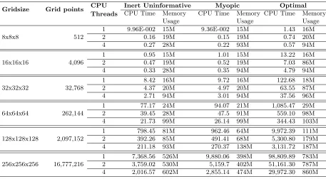
Table 1 reports runtimes and memory usage of CPU-based computations for the three types of policies. These were implemented in Fortran90 with outermost loop over the state space explicitly parallelized using OpenMP directives (Chandra, Menon, Dagum, and Kohr,
7Preliminary efforts to ensure robustness of minimization step involved testing our method against
2000; Chapman, Jost, and van der Paas, 2007). The code was compiled in double precision8 with Intel Fortran compiler for 64-bit systems, version 11.0,9and run on a high performance quad-core single CPU workstation utilizing Core i7 Extreme Edition 965 Nehalem CPU overclocked to 3.4 GHz. In order to reduce timing noise, the codes were run four times and compute times averaged out for each policy type, CPU thread count and gridsize. It should be clear that the deck is intentionally stacked in CPU favor.
Table 1 serves to emphasize very good scaling of numerical dynamic programming with the thread count, since communication among different threads is not required and workload per thread is fairly uniform. For small grid sizes overhead of thread creation and destruction dominates performance benefit of multiple threads.10 At large grid sizes, memory becomes
limiting factor both in terms of ability to store cost-to-go function and to quickly update it in memory.
Gridsize Grid points CPU Threads
Inert Uninformative Myopic Optimal
CPU Time Memory Usage
CPU Time Memory Usage
CPU Time Memory Usage
8x8x8 512
1 9.96E-002 15M 9.36E-002 15M 1.43 16M 2 0.16 19M 0.15 19M 0.74 20M 4 0.27 28M 0.22 93M 0.57 94M
16x16x16 4,096
1 0.95 15M 1.01 15M 13.22 16M 2 0.47 19M 0.52 19M 7.03 86M 4 0.33 28M 0.35 94M 4.79 94M
32x32x32 32,768
1 8.42 16M 9.72 16M 122.68 18M 2 4.37 20M 4.97 20M 63.55 87M 4 2.71 94M 3.01 94M 37.56 96M
64x64x64 262,144
1 77.17 24M 94.07 21M 1,085.47 29M 2 39.45 28M 47.5 91M 559.10 98M 4 21.73 99M 26.14 99M 344.43 103M
128x128x128 2,097,152
1 798.45 81M 962.46 64M 9,972.39 111M 2 392.26 85M 491.41 68M 5,300.80 179M 4 211.18 93M 270.37 138M 3,131.72 187M
256x256x256 16,777,216
[image:10.612.80.537.272.524.2]1 7,368.56 526M 9,880.06 398M 98,809.89 783M 2 3,759.02 530M 5,159.7 402M 51,161.30 787M 4 2,016.57 602M 2,855.14 474M 29,972.30 860M
Table 1: Performance scaling of CPU-based computation under different policies
4.2. GPU-based computation. For our GPU-based computations we used graphics card featuring GTX280 chip. It has 1.4 billion transistors, theoretical peak performance of 933 Gflops in single precision, peak memory bandwidth of 141.7 Gb/sec and capability to work on 30,720 threads simultaneously.11
GPU-based computation mirrors CPU-based one in all respects except for how it dis-tributes the work across multiple threads. Code fragments below illustrate the differences
8Same code compiled in single precision required more dynamic programming iterations to achieve
con-vergence to the same tolerance, outweighing speed benefits of lower precision.
9Intel compilers (Fortran and C) performed significantly better then those from GNU complier collection
(gccandgfortran).
10More elaborate performance-oriented implementation would vary number of threads depending on the
size of the problem in order to avoid performance degradation due to thread creation.
in the implementation of the main sweep over all point on the grid between the two program-ming frameworks. To focus on the key details, we selected these fragments from a codebase for the evaluation of the cost-to-go function of the cautionary myopic policy. The code for the optimal policy is conceptually similar but is obscured by the details of implementing the minimization operator. We also omit parts of the code that are not interesting, such as checking iteration progress, reading input or generating output files. Omitted segments are marked by ellipses.
Fortran 90 code 1 ...
2 ! set multithreaded OpenMP version using all available CPUs 3 #ifdef _OPENMP
4 call OMP_SET_NUM_THREADS(numthreads) 5 #endif
6 allocate(V(NX,Nmu,NSigma,2),U(NX,Nmu,NSigma)) 7 ...
8 supval = abs(10.0d0*PolTol+1.0) 9 polit1=0
10 ip = 1 11 ppass =0
12 do while((ip<MaxPolIter+1).and.(ppass.eq.0)) 13 ! loop over the grid of the three state variables 14 !$omp parallel default(none) &
15 !$omp shared(NX,Nmu,NSigma,U,V,X,mu,Sigma,alpha,gamma,delta,omega,ustar,xstar,sigmasq_epsilon) & 16 !$omp private(i,j,k)
17 !$omp do 18 do i=1,NX 19 do j=1,Nmu 20 do k=1,NSigma
21 V(i,j,k,2) = F(U(i,j,k),i,j,k,V)
22 enddo
23 enddo 24 enddo 25 !$omp end do 26 !$omp end parallel 27
28 ! check convergence criterion for the policy function iteration 29 supval = maxval(abs(V(:,:,:,1)-V(:,:,:,2)))
30 checkp = maxval(delta*abs(V(:,:,:,1)-V(:,:,:,2))/((1-delta)*(abs(V(:,:,:,1))))) 31 if (checkp<PolTol) then
32 ppass = 1 33 endif 34
35 ! update the value function 36 V(:,:,:,1) = V(:,:,:,2) 37
38 print *, ’ FINISHED POlICY ITERATION’,ip 39 if (ppass.eq.1) then
40 print *, ’POLICY ITERATION CONVERGED’ 41 else
42 print *, ’POLICY ITERATIONS - NO CONVERGENCE’ 43 endif
44 ip=ip+1 45 enddo 46 polit1=ip-1 47 ...
The Fortran code is fairly straightforward. The main loop starts on line 14 and encloses pointwise value updates. So called OpenMPsentinelson lines 14-17 and 25-26 tell compiler to generate multiple threads that will execute the loop in parallel. Division of the workload is up to compiler to decide.
Cuda code (main) 1 ...
2 cudaMalloc((void**) &d_X,NX*sizeof(double)); 3 ...
4 cudaMemcpy(d_X,X,NX*sizeof(double),cudaMemcpyHostToDevice); 5 ...
6 numBlocks=512; 7 numThreadsPerBlock=180; 8 dim3 dimGrid(numBlocks);
11 // start value iteration cycles 12 supval=fabs(10.0*PolTol+1.0); 13 polit1=0;
14 ip=1; 15 ppass=0;
16 while ((ip<MaxPolIter+1)&&(ppass==0))
17 {
18
19 // update expected cost-to-go function on the whole grid (in parallel)
20 UpdateExpectedCTG_kernel<<<dimGrid,dimBlock>>>(d_U,d_X,d_mu,d_Sigma,d_V0,d_rno,d_wei,d_V1); 21 cudaThreadSynchronize();
22
23 // move the data from device to host to do convergence checks
24 cudaMemcpy(V1,d_V1,NX*Nmu*NSigma*sizeof(double),cudaMemcpyDeviceToHost); 25
26 // check convergence criteria for the policy function iteration if ip>=2 27 ...
28 // update value function, directly on the device
29 cudaMemcpy(d_V0,d_V1,NX*Nmu*NSigma*sizeof(double),cudaMemcpyDeviceToDevice); 30 // update value function on host as well
31 cudaMemcpy(V0,V1,NX*Nmu*NSigma*sizeof(double),cudaMemcpyHostToHost); 32 ...
33 }
34 ...
35 cudaFree(d_X); 36 ...
CUDA code requires separate memory spaces allocated on the host CPU and on the graphics device, with explicit transfers between the two. It replaces entire loop with a call to a kernel function (line 20). Kernel function is executed by each thread applying device function to its own chunk of data. The number of threads and their organization into blocks of threads is an important tuning parameter. More threads in a block hide memory latencies better but it will also reduce resources available to each thread. For a rough guidance on the tradeoff between the size and the number of blocks we used NVIDIA’s CUDA occupancy calculator, a handy spreadsheet tool. Additionally, all the model parameters as well as fixed quantities such as gridsizes or convergence tolerances were placed in constant memory to facilitatelocal access to these values by each thread. No further optimizations were initially applied. The final code snippet shows some internals of the kernel code but omits device function. Internals of the device function are functionally identical to similar Fortran code and perform Gauss-Hermite integration of tri-linearly interpolated value function.
Cuda kernel code 1 ...
2 __device__ inline double UpdateExpectedCTG(double u, double x, double mu, double Sigma, 3 double alpha, double gamma, double delta, double omega, double sigmasq_epsilon, 4 double xstar, double ustar, int NX,int Nmu, int NSigma, int NGH, double* XGrid, 5 double* muGrid, double* SigmaGrid, double* V, double* rno, double* wei); 6 __global__ void UpdateExpectedCTG_kernel(double* U,double* X,double* mu, 7 double* Sigma,double* V0,double* rno,double* wei,double* V1)
8 {
9
10 //Thread index
11 const int tid = blockDim.x * blockIdx.x + threadIdx.x; 12 const int NUM_ITERATION= dc_NX*dc_Nmu*dc_NSigma;
13 int ix,jmu,kSigma; 14
15 //Total number of threads in execution grid 16 const int THREAD_N = blockDim.x * gridDim.x; 17
18 //ech thread works on as many points as needed to update the whole array 19 for (int i=tid;i<NUM_ITERATION;i+=THREAD_N)
20 {
21 //update expected cost-to-go point-by-point 22 ix=i/(dc_NSigma*dc_Nmu);
23 jmu=(i-ix*dc_Nmu*dc_NSigma)/dc_NSigma; 24 kSigma=i-ix*dc_Nmu*dc_NSigma-jmu*dc_NSigma;
25 V1[i]=UpdateExpectedCTG(U[i],X[ix],mu[jmu],Sigma[kSigma],dc_alpha, 26 dc_gamma,dc_delta,dc_omega,dc_sigmasq_epsilon,dc_xstar,dc_ustar, 27 dc_NX,dc_Nmu,dc_NSigma,dc_NGH,X,mu,Sigma,V0,rno,wei);
29 30 } 31 ...
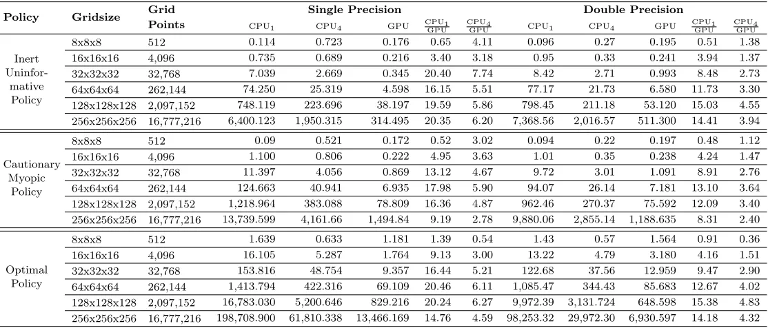
4.3. Speed comparison. Table 2 documents initial timing results for GPU implementa-tions in single and double precision in comparison to single-threaded and multi-threaded CPU-based implementation. These are done for all three policies and across a range of grid-sizes. As with CPU-based implementation, CUDA codes were time several time to reduce measurement noise.
Several things are worth noticing in table 2. First is that across all cases, GPU wins over single CPU in 86% of cases, and over four cores in 94% of cases. GPU only loses for the smallest problem sizes, where multithreading, whether based on CPU or GPU, is actually detrimental to performance due to thread creation and destruction overheads. Second, the margin of victory is oftentimes quite substantial, in some more than factor of 20. Third, single precision calculation on the GPU is generally faster than in double precision, especially taking into consideration that dynamic programming algorithm takes up to 50% more iterations to converge in single precision, with exactly ratio depending on gridsize and policy type. In contrast, the speed of single precision calculation on the CPU is only marginally different from double precision, after accounting for convergence effect. This is because GPUs have separate units dedicated to double and single precision floating point calculations but CPUs do not. Moreover, current generation of Nvidia GPUs has only 1/8 as many resources devoted to double precision as to single precision work. With this in mind, it is actually surprizing how little difference there is between double and single precision results on GPU. This is likely due to underutilization of floating point resources in either case.
Policy Gridsize Grid Points
Single Precision Double Precision
CPU1 CPU4 GPU CPU1GPU CPU4GPU CPU1 CPU4 GPU CPU1GPU CPU4GPU
Inert
Uninfor-mative Policy
8x8x8 512 0.114 0.723 0.176 0.65 4.11 0.096 0.27 0.195 0.51 1.38 16x16x16 4,096 0.735 0.689 0.216 3.40 3.18 0.95 0.33 0.241 3.94 1.37 32x32x32 32,768 7.039 2.669 0.345 20.40 7.74 8.42 2.71 0.993 8.48 2.73 64x64x64 262,144 74.250 25.319 4.598 16.15 5.51 77.17 21.73 6.580 11.73 3.30 128x128x128 2,097,152 748.119 223.696 38.197 19.59 5.86 798.45 211.18 53.120 15.03 4.55 256x256x256 16,777,216 6,400.123 1,950.315 314.495 20.35 6.20 7,368.56 2,016.57 511.300 14.41 3.94
Cautionary Myopic
Policy
8x8x8 512 0.09 0.521 0.172 0.52 3.02 0.094 0.22 0.197 0.48 1.12
16x16x16 4,096 1.100 0.806 0.222 4.95 3.63 1.01 0.35 0.238 4.24 1.47 32x32x32 32,768 11.397 4.056 0.869 13.12 4.67 9.72 3.01 1.091 8.91 2.76 64x64x64 262,144 124.663 40.941 6.935 17.98 5.90 94.07 26.14 7.181 13.10 3.64 128x128x128 2,097,152 1,218.964 383.088 78.809 16.36 4.87 962.46 270.37 75.592 12.09 3.40 256x256x256 16,777,216 13,739.599 4,161.66 1,494.84 9.19 2.78 9,880.06 2,855.14 1,188.635 8.31 2.40
Optimal Policy
8x8x8 512 1.639 0.633 1.181 1.39 0.54 1.43 0.57 1.564 0.91 0.36
[image:13.612.32.589.414.652.2]16x16x16 4,096 16.105 5.287 1.764 9.13 3.00 13.22 4.79 3.180 4.16 1.51 32x32x32 32,768 153.816 48.754 9.357 16.44 5.21 122.68 37.56 12.959 9.47 2.90 64x64x64 262,144 1,413.794 422.316 69.109 20.46 6.11 1,085.47 344.43 85.683 12.67 4.02 128x128x128 2,097,152 16,783.030 5,200.646 829.216 20.24 6.27 9,972.39 3,131.724 648.598 15.38 4.83 256x256x256 16,777,216 198,708.900 61,810.338 13,466.169 14.76 4.59 98,253.32 29,972.30 6,930.597 14.18 4.32
Table 2: Runtime comparison of CPU and GPU-based calculations.
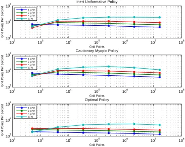
to memory limitations. In contrast, the performance of two- and four-threaded versions of the two suboptimal policies initially improves with problem size as fixed costs of multiple threads are spread over longer runtime but starts to fall relatively early. More complex calculation per grid point for the optimal policy causes the downward trend in performance throughout the entire gridsize range. GPU performance, on the other hand, continues to improve until moderately large grid size but still drops for the very large grids.
102 103 104 105 106 107 108
102
104
106
Grid Points
Grid Points Per Second
Inert Uniformative Policy
1 CPU 2 CPU 4 CPU GPU
102 103 104 105 106 107 108
102
104
106
Grid Points
Grid Points Per Second
Cautionary Myopic Policy
1 CPU 2 CPU 4 CPU GPU
102 103 104 105 106 107 108
102
104
106
Grid Points
Grid Points Per Second
Optimal Policy
[image:14.612.140.506.208.499.2]1 CPU 2 CPU 4 CPU GPU
Figure 1: Speed comparison of CPU and GPU-based approaches for double precision calcu-lations.
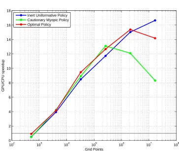
Figure 4.3 distills performance numbers further by focusing on the GPU speedup ratio relative to the single CPU. It emphasizes two things – somewhat limited applicability of GPU speedups and substantial speed boost for moderately sized grids even for double precision. Beyond the optimal problem size the drop in speed can be precipitous.12
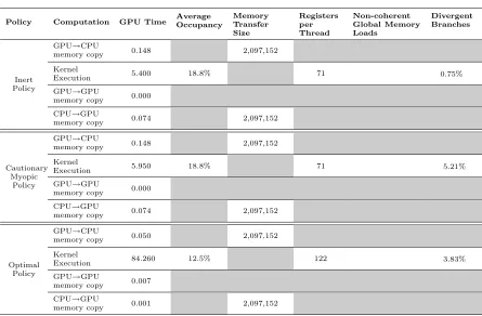
To see if our code can benefit from further performance tuning we made use of CUDA profiler tool. Results are reported in table 3.
Average occupancy of about 10-20% indicates that only 3-6 thousands of threads can be launched simultaneously (out of 30 thousand) with enough resources. Potentially, a speedup on the order of 5-10 factor remains unrealized. Specifically, the limiting resource is the number of registers, a type of very fast on-chip memory used to store intermediate
102 103 104 105 106 107 108 0
2 4 6 8 10 12 14 16 18
Grid Points
GPU/CPU speedup
[image:15.612.140.504.103.410.2]Inert Uniformative Policy Cautionary Myopic Policy Optimal Policy
Figure 2: Ratio of GPU and single CPU speeds for double precision calculations.
calculations. CUDA toolkit provides a compiler switch to limit the register use at a cost of larger machine code. We will investigating the usefulness of the switch next.
Divergent branches refer to situations when different threads within the same groups for threads called warp take different paths following a branch condition. Thread divergence leads to performance degradation. Fortunately, for our code the incidence of divergent branches is low.
5. Concluding Remarks
Policy Computation GPU Time AverageOccupancy MemoryTransfer Size
Registers per Thread
Non-coherent Global Memory Loads
Divergent Branches
Inert Policy
GPU→CPU
memory copy 0.148 2,097,152 Kernel
Execution 5.400 18.8% 71 0.75% GPU→GPU
memory copy 0.000 CPU→GPU
memory copy 0.074 2,097,152
Cautionary Myopic
Policy
GPU→CPU
memory copy 0.148 2,097,152 Kernel
Execution 5.950 18.8% 71 5.21% GPU→GPU
memory copy 0.000 CPU→GPU
memory copy 0.074 2,097,152
Optimal Policy
GPU→CPU
memory copy 0.050 2,097,152 Kernel
Execution 84.260 12.5% 122 3.83% GPU→GPU
memory copy 0.007 CPU→GPU
[image:16.612.83.528.109.401.2]memory copy 0.001 2,097,152
Table 3: CUDA Profiler report based on runs with 64x64x64 gridsize.
Development of parallel computing on GPU is bound to have an impact on high per-formance computing industry as graphics cards are already inexpensive and ubiquitous. Indeed, with peak performance of nearly one teraflop, the compute power of today’s graph-ics processors dwarfs that of the commodity CPU while costing only a few hundred dollars. If nothing else, emergence of GPU as a viable competitor to traditional CPU for high perfor-mance computing will elicit a response by major CPU manufacturers, a duopoly of Intel and AMD. Even though CPU development may appear positively glacial compared to quantum performance leaps in GPUs, nothing prevents CPUs from adopting ideas of data parallel processing. CPUs are growing to have more cores, capable of more threads, add special units for streaming and vector computations. Already, many-core CPU and GPU hybrids are in development. For example, Intel has publicly acknowledged working on Larrabee project to compete in GPGPU and high performance computing markets (Seiler, Carmean, Sprangle, Forsyth, Abrash, Dubey, Junkins, Lake, Sugerman, Cavin, Espasa, Grochowski, Juan, and Hanrahan, 2008). This new architecture is promised to resemble the well known programming model for x86 multi-core architectures, so that many C/C++ applications can be simply recompiled for Larrabee and execute correctly with no code modification. This application portability, together with ability to hide low-level details from programmer,13
could be produce large performance gains without extreme algorithmic effort. Whether this promise is realized will be a subject of further research.
In the end, it doesn’t matter whether GPUS will merge into CPUs or vice versa. What does matter is how to harness the raw power of data-parallel approach for general purpose computations. Development of programming tools is essential here and the effort is already
13For example, unlike CUDA, Larrabee does not require direct management of data movement among
well under way. Among other things, compiler vendors are working on inclusion of GPU accelerator technology with their Fortan and C compilers. For example, using provisional support by PGI Group (The Portland Group, 2008), programmers will be able to accelerate Linux applications by adding OpenMP-like compiler directives that instruct the compiler to analyze the whole program structure and data, split portions of the applications between CPU and GPU as specified by user directives, and define and generate an optimized mapping of loops to automatically use the parallel cores, hardware threading capabilities and SIMD vector capabilities of modern GPUs.
The future of many computations belongs to parallel algorithms. Today’s era of tra-ditional von Neumann sequential programming model (Backus, 1977) with its escalating disparity between the high rate at which CPU can work and limited data throughput between it and memory is nearly over. Modern processors are becoming wider but not faster. The change in computational landscape presents both challenges and opportunities for economists and financial engineers. Our paper is but a modest attempt to pick up low hanging fruit.
References
Abdelkhalek, A., A. Bilas, and A. Michaelides (2001): “Parallelization, optimiza-tion and performance analysis of portfolio choice models,” in Proceedings of the 2001 International Conference on Parallel Processing (ICPP01).
Backus, J. (1977): “Can Programming be Liberated from the von Neumann Style?,” Communications of the ACM, 21(8), 613–641.
Bargen, B., and P. Donnelly (1998): Inside DirectX, Microsoft Programming Series. Microsoft Press, Redmond, Washington.
Beck, G. W., and V. Wieland (2002): “Learning and control in a changing economic environment,”Journal of Economic Dynamics and Control, 26(9-10), 1359–1377. Bennemann, C., M. W. Beinker, D. Eggloff, and M. Guckler (2008): “Teraflops
for Games and Derivatives Pricing,”Wilmott Magazine, pp. 50–54.
Bertsekas, D. P. (2001): Dynamic Programming and Optimal Control, vol. 2. Athena Scientific, Nashua, NH, 2 edn.
(2005): Dynamic Programming and Optimal Control, vol. 1. Athena Scientific, Nashua, NH, 3 edn.
Brent, R. P. (1973): Algorithms for Minimization without Derivatives. Prentice-Hall, Englewood Cliffs.
Brezzia, M., and T. L. Lai (2002): “Optimal learning and experimentation in bandit problems,”Journal of Economic Dynamics and Control, 27(1), 87–108.
Buck, I.(2005): “Stream computing on graphics hardware,” Ph.D. Dissertation, Stanford University, Stanford, CA, USA.
Chandra, R., R. Menon, L. Dagum, and D. Kohr (2000): Parallel Programming in OpenMP. Morgan Kaufmann.
Chapman, B., G. Jost,and R. van der Paas(2007): Using OpenMP: Portable Shared Memory Parallel Programming, Scientific and Engineering Computation Series. MIT Press, Cambridge, MA.
Chong, Y. Y., and D. F. Hendry (1986): “Econometric Evaluation of Linear Macro-economic Models,”The Review of Economic Studies, 53(4), 671–690.
Coleman, W. J. (1992): “Solving Nonlinear Dynamic Models on Parallel Computers,” Discussion Paper 66, Institute for Empirical Macroeconomics, Federal Reserve Bank of Minneapolis.
Creel, M. (2005): “User-Friendly Parallel Computations with Econometric Examples,” Computational Economics, 26(2), 107–128.
Creel, M., andW. L. Goffe(2009): “Multi-core CPUs, Clusters, and Grid Computing: A Tutorial,”Computational Economics, p. forthcoming.
Doornik, J. A., D. F. Hendry, andN. Shephard (2002): “Computationally-intensive econometrics using a distributed matrix-programming language,”Philosophical Transac-tions of the Royal Society of London, Series A, 360, 1245–1266.
Doornik, J. A., N. Shephard, and D. F. Hendry (2006): “Parallel Computation in Econometrics: A Simplified Approach,” inHandbook of Parallel Computing and Statistics, pp. 449–476. Chapman & Hall/CRC.
Easley, D., andN. M. Kiefer(1988): “Controlling a Stochastic Process with Unknown Parameters,”Econometrica, 56(5), 1045–1064.
Ferrall, C.(2003): “Solving Finite Mixture Models in Parallel,” Computational Econom-ics 0303003, EconWPA.
Goffe, W. L., G. D. Ferrier,andJ. Rogers(1994): “Global optimization of statistical functions with simulated annealing,”Journal of Econometrics, 60(1-2), 65–99.
Goldberg, D. E.(1989): Genetic Algorithms in Search, Optimization and Machine Learn-ing. Addison-Wesley, Reading, MA.
Gropp, W., E. Lusk, A. Skjellum,andR. Thakur(1999): Using MPI: Portable Paral-lel programming with Message Passing Interface, Scientific and Engineering Computation Series. MIT Press, Cambridge, MA, 2 edn.
Horst, R.,andP. M. Paradalos (eds.) (1994): Handbook of Global Optimization, vol. 1 ofNonconvex Optimization and Its Applications. Kluwer Academic Publishers, Dordrecht, The Netherlands.
Judge, G. G., T.-C. Lee,andR. C. Hill(1988): Introduction to the Theory and Practice of Econometrics. Wiley, New York, 2 edn.
Kendrick, D. A. (1978): “Non-convexities from probing an adaptive control problem,” Journal of Economic Letters, 1(4), 347–351.
Kessenich, J., D. Baldwin, and R. Rost (2006): The OpenGL Shading
Lan-guageKhronos Group.
Kirk, D., andW. Hwu(2009): CUDA Programming.
Kirkpatrick, S., C. D. Gelatt Jr., and M. P. Vecchi (1983): “Optimization by Simulated Annealing,”Science, 220(4598), 671–680.
Kola, K., A. Chhabra, R. K. Thulasiram, and P. Thulasiraman(2006): “A Soft-ware Architecture Framework for On-line Option Pricing,” inProceedings of the 4th Inter-national Symposium on Parallel and Distributed Processing and Applications (ISPA-06), vol. 4330 ofLecture Notes in Computer Science, pp. 747–759, Sorrento, Italy. Springer-Verlag.
Lagarias, J. C., J. A. Reeds, M. H. Wright,andP. E. Wright(1998): “Convergence Properties of the Nelder-Meade Simplex Method in Low Dimensions,”SIAM Journal of Optimization, 9(1), 112–147.
Lewis, R. M., and V. Torczon (2002): “A Globally Convergent Augmented La-grangian Pattern Search Algorithm for Optimization with General Constraints and Simple Bounds,”SIAM Journal on Optimization, 12(4), 1075–1089.
Lindoff, B., and J. Holst (1997): “Suboptimal Dual Control of Stochastic Systems with Time-Varying Parameters,” mimeo, Department of Mathematical Statistics, Lund Institute of Technology.
Morozov, S. (2008): “Learning and Active Control of Stationary Autoregression with Unknown Slope and Persistence,” Working paper, Stanford University.
(2009a): “Bayesian Active Learning and Control with Uncertain Two-Period Im-pulse Response,” Working paper, Stanford University.
Nagurney, A., T. Takayama,andD. Zhang(1995): “Massively parallel computation of spatial price equilibrium problems as dynamical systems,”Journal of Economic Dynamics and Control, 19(1-2), 3–37.
Nagurney, A.,and D. Zhang(1998): “A massively parallel implementation of discrete-time algorithm for the computation of dynamic elastic demand and traffic problems mod-eled as projected dynamical systems,”Journal of Economic Dynamics and Control, 22(8-9), 1467–1485.
Nelder, J. A., and R. Mead (1965): “A simplex method for function minimization,” Computer Journal, 7, 308–313.
NVIDIA Corporation (2008): NVIDIA CUDA Compute Unified Device Architecture: Programming Guide NVIDIA Corporation, Santa Clara, CA, 2 edn.
Paradalos, P. M., andH. E. Romeijn (eds.) (2002): Handbook of Global Optimization, vol. 2 of Nonconvex Optimization and Its Applications. Kluwer Academic Publishers, Dordrecht, The Netherlands.
Pflug, G. C., and A. Swietanowski (2000): “Selected parallel optimization methods for financial management under uncertainty,”Parallel Computing, 26(1), 3–25.
Prescott, E. C.(1972): “The Multi-Period Control Problem Under Uncertainty,” Econo-metrica, 40(6), 1043–1058.
Rahman, M. R., R. K. Thulasiram, and P. Thulasiraman (2002): “Forecasting Stock Prices using Neural Networks on a Beowulf Cluster,” in Proceedings of the Four-teenth IASTED International Conference on Parallel and Distributed Computing and Sys-tems (PDCS 2002), ed. by S. Akl, and T.Gonzalez, pp. 470–475, Cambridge, MA USA. IASTED, MIT Press.
Seiler, L., D. Carmean, E. Sprangle, T. Forsyth, M. Abrash, P. Dubey, S. Junk-ins, A. Lake, J. Sugerman, R. Cavin, R. Espasa, E. Grochowski, T. Juan,and
P. Hanrahan (2008): “Larrabee: A Many-Core x86 Architecture for Visual Comput-ing,”ACM Transactions on Graphics, 27(3), 15 pages.
Sims, C. A., D. F. Waggoner,andT. Zha(2009): “Methods for Inference in Large-Scale Multiple Equation Markov-Switching Models,”Journal of Econometrics, forthcoming. Spendley, W., G. R. Hext, and F. R. Himsworth(1962): “Sequential application of
simplex designs in optimization and evolutionary design,”Technometrics, 4, 441–461. Svensson, L. E. O.(1997): “Optimal Inflation Targets, ’Conservative’ Central banks, and
Linear Inflation Contracts,”American Economic Review, 87(1), 96–114.
Swann, C. A. (2002): “Maximum Likelihood Estimation Using Parallel Computing: An Introduction to MPI,”Computational Economics, 19(2), 145–178.
The Portland Group(2008):PGI Fortran & C Accelerator Compilers and Programming Model Technology PreviewThe Portalnd Group, Version 0.7.
Wieland, V. (2000): “Learning by Doing and the Value of Optimal Experimentation,” Journal of Economic Dynamics and Control, 24(4), 501–535.
Zabinsky, Z. B.(2005): Stochastic Adaptive Search for Global Optimization. Springer. Zenios, S. A.(1999): “High-performance computing in finance: The last 10 years and the
next,”Parallel Computing, 25(13-14), 2149–2175.