Image Processing Techniques in Shockwave Detection and
Modeling
Suxia Cui1, Yonghui Wang2, Xiaoqing Qian3, Zhengtao Deng3
1
Department of Electrical and Computer Engineering, Prairie View A&M University, Prairie View, Texas, USA; 2Department of Engineering Technology, Prairie View A&M University, Prairie View, Texas, USA; 3Department of Mechanical Engineering, Ala- bama A&M University, Huntsville, Alabama, USA.
Email: [email protected], [email protected], [email protected], [email protected]
Received May, 2013.
ABSTRACT
Shockwave detection is critical in analyzing shockwave structure and location. High speed video imaging systems are commonly used to obtain image frames during shockwave control experiments. Image edge detection algorithms be- come natural choices in detecting shockwaves. In this paper, a computer software system designed for shockwave de- tection is introduced. Different image edge detection algorithms, including Roberts, Prewitt, Sobel, Canny, and Lapla- cian of Gaussian, are implemented and can be chosen by the users to easily and accurately detect the shockwaves. Ex- perimental results show that the system meets the design requirements and can accurately detect shockwave for further analysis and applications.
Keywords: Shock Wave Detection; Image Edge Detection
1. Introduction
A shockwave is a strong compression wave existing in supersonic/hypersonic flow field. Across the shockwave gas pressure, temperature and density increases signifi- cantly as a function of flow Mach number. Near the nose area of a supersonic/hypersonic flight vehicle, strong shockwaves exist. Extreme heat fluxes and heat load to the vehicle surface requires strong thermal protection in the nose area. Additionally, the shock standoff distance varies drastically with the temperature for a non-ideal gas, causing large differences in the heat transfer to the ther- mal protection system and drag of the vehicle. Super- sonic wind tunnel experiments are needed to provide insight into the physics of air flow at high Mach numbers. Knowing the location and shape of the shockwave is es- sential to the success of vehicle design. In general, opti- cal imaging system can be used to capture shockwave shape, location and flow property changes near the test article in a supersonic wind tunnel. High speed video imaging system and Schlieren system will normally gen- erate significant amount of images that need to be ana- lyzed after the experiment. Image processing techniques can make this type of data analysis more efficient and precise, but there exists challenges on how to pre-process the obtained images according to the wind tunnel condi- tion as well as dealing with large volume of data cap tured by high speed camera. Data acquisition is
per-formed in wind tunnel, while data analysis will be com- pleted by a powerful PC.
2. Shockwave Stand-off Distance Detection
A series of shockwave control experiments were con- ducted using a supersonic wind tunnel facility. The su- personic flow is created by a primary supersonic nozzle to provide supersonic speed up to Mach 4. The flow emerging from the nozzle is then exhausted as a free jet into a windowed low pressure test cabin with extremely low back pressure. Figure 1 shows the shockwave ex- periment setting and a typical experimental image cap- tured by a high speed video camera for a Mach 4 shock- wave control experiment. The test article basic diameter (perpendicular to the incoming flow direction) is 3cm and the nose is spherical. The length of the cylindrical part is around 7 cm with the total length of the model from nose tip to cylinder base is 10cm. The shockwave structure and location capturing device were captured by a high speed video imaging system with speed of 2000 frames per second at 512 x 512 resolutions. Around 8000 frames of image data was collected for each experi- ment.
shape change of the shockwave especially the shockwave stand-off distance along the stagnation line. Since the experimental image has built-in noise, a noise cancella- tion algorithm should be incorporated in the detection scheme. The detection algorithm should also be robust because the large amount of unsteady shockwave images has to be analyzed. The time history of the shockwave stand-off distance under control conditions has to be pre- cisely captured.
Figure 1. Aero-Test Article inside the wind tunnel and typical shockwave image near the nose are of the test arti- cle.
The current research focused on the development of a new shockwave standoff distance detection algorithm. To detect the shockwave shape and stand-off distance through the images, image processing techniques can be used to make this type of data analysis more efficient and precise. In the current research, a new interactive and user-friendly shockwave detection software was devel- oped. This software can precisely detect the shockwave stand-off distance in front of the test article inside a su- personic wind tunnel.
3. Image Edge Detection Algorithms
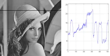
Edge detection algorithm is the natural choice for detect- ing shockwave within the obtained high speed video se- quences. Edges are local features of images, which are local regions with special properties. Edges are pixels with significant local changes of intensity–large gradi- ent–in an image. Edges typically occur on the boundary between two different regions in an image (as shown in
Figure 2). Because important features, such as corners, lines, curves, etc., can be extracted from the edges, edge detection algorithms are very important in computer vi- sion applications. Edge detection is to detect the edges and to produce a line drawing of a scene from an image of that scene.
There are four steps for edge detection: (1) Smoothing: suppress as much noise as possible, without destroying the true edges. (2) Enhancement: apply a filter to en- hance the quality of the edges in the image (sharpening).
(3) Detection: determine which edge pixels should be discarded as noise and which should be retained (usually, thresholding provides the criterion used for detection). (4) Localization: determine the exact location of an edge Edge thinning and linking are usually required in this step.
Figure 2. Image edge example: a scan line highlighted (left) and intensity along the highlighted scan line (right).
In mathematics, derivatives are used to describe changes of continuous functions. Applying this to 2D images, partial derivatives can be used to express the image intensity changes (e.g. edges). Edge points can be detected by detecting (1) the local maxima or minima of the first derivative and (2) the zero-crossing of the sec-ond derivative. For 1D discrete signals, the first deriva-tive can be approximated as
0
( )
lim 1 ( )
a
f x a f x
f x f
a
x f x ;
and the second derivative can be approximated as
0
lim
a
f x f x a
f x
a
1
f x f x
( 1) 2 ( ) ( 1)
f x f x f x
.
For 2D images, gradient can be used to describe edges. Gradient is defined as a vector
[ f , f]
f
x y
,
its magnitude,
2 2
( f) ( f)
f
x y
,
provides the edge’s strength information. For images, by using pixel-coordinate notation (e.g., for row number and for column number, and
i
j I for image signal), the gradient can be approximated as
0
, ,
lim 1, ,
a
I x a y I x y
I
I x y I x y
x a
( , 1) ( , )
I i j I i j
, and
0
( , ) ( , )
lim ( , 1) ( , )
a
I I x y a I x y
I x y I x y
y a
( 1, ) ( , )
I i j I i j
[image:2.595.74.269.204.328.2]3.1. Roberts
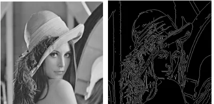
The Roberts method finds edges using the Roberts approximation to the derivative. It returns edges at those points where the gradient of I is maximum. It was one of the first edge detectors and was initially proposed by Lawrence Roberts [1]. The Roberts edge detector ap- proximates the partial derivatives of the gradient as
, 1,I
I i j I i j
x
1
,
1,
, 1
II i j I i j
y
.
This approximation can be implemented by convolving the following masks
1 0 0 1
x M
and 0 1
1 0
y
M
[image:3.595.317.530.84.188.2]onto images. An example of Roberts edge detection is shown in Figure 3.
Figure 3. Roberts edge detector: original image (left) and detected edges (right).
3.2. Prewitt
The Prewitt method finds edges using the Prewitt ap- proximation to the derivative. It was proposed by Judith M. S. Prewitt [2]. The Prewitt operator approximates the partial derivatives of the gradient as
1, 1
, 1
1, 1I
I i j I i j I i j
x
1, 1
( , 1) ( 1, 1)I i j I i j I i j
,
1, 1
1,
1, 1I
I i j I i j I i j
y
1, 1
( 1, ) ( 1, 1)I i j I i j I i j
.
The approximation can be implemented by convolving the following masks
1 0 1 1 0 1 1 0 1
x M
and
1 1 1 0 0 0 1 1 1
y M
[image:3.595.66.280.341.447.2]onto images. An example of Prewitt edge detection is shown in Figure 4.
Figure 4. Prewitt edge detector: original image (left) and detected edges (right).
3.3. Sobel
The Sobel method finds edges using the Sobel approxi-mation to the derivative. It was proposed by Irwin E. Sobel in 1970 [3]. A little bit different from the Prewitt operator, the Sobel operator approximates the partial derivatives of the gradient as
1, 1
2
, 1
1, 1I
I i j I i j I i j
x
1, 1
2 ( , 1) ( 1, 1)I i j I i j I i j
,
1, 1
2
1,
1, 1I
I i j I i j I i j
y
1, 1
2 ( 1, ) ( 1, 1)I i j I i j I i j
.
The approximation can be implemented by convolving the following masks
1 0 1 2 0 2 1 0 1
x M
and
1 2 1 0 0 0 1 2 1
y M
onto images. An example of Sobel edge detection is shown in Figure 5.
Figure 5. Sobel edge detector: original image (left) and de-tected edges (right).
Edge detection algorithms with Roberts, Prewitt, and Sobel operators share the same procedure in detecting edges. Main steps in edge detection with these operators: (1) calculate partial derivatives of the image through
convolution, x * x I
I I M
x
and y * y
I
I I M
y
; (2)
[image:3.595.318.530.502.606.2]2
( I) ( I)2
I
x y
; and (3) if I i j( , ) T, then it
is possible an edge point, T is the threshold.
3.4. Canny
Also being a method which finds edges by looking for local maxima of the gradient of the image, the Canny algorithm, which was developed by John F. Canny in 1986 [4], introduces more steps to minimize the noise affection. To reduce the noise effect, a low-pass Gaus- sian filter,
2 2
2
2 2
1 ,
2
x y
G x y e
, (1)
is applied to the image. By finding the derivative of the Gaussian filter, the gradient can be calculated
*
* *x x
I
I I G I G I G
x x x
,
*
* *y I
x
I I G I G I G
x x x
,
where Gx x2G x( , )
y and Gy y2G x( , )
y .
After the gradient magnitude, I Ix2Iy2, is ob-
[image:4.595.56.288.241.376.2] [image:4.595.318.529.380.484.2]tained, two more steps are performed to identify the edges. A non-maxima suppression algorithm is applied to find the local maxima of the gradient magnitude, and a hysteresis thresholding with two thresholds is applied to get rid of extra noise and retain the real edge points. This method is therefore less likely than the others to be fooled by noise, and more likely to detect true weak edges. An example of Canny edge detection is shown in
Figure 6.
Figure 6. Canny edge detector: original image (left) and detected edges (right).
3.5. Laplacian of Gaussian
The Laplacian of Gaussian (LoG) method identifies edges by looking for zero crossings after filtering the image with an LoG filter [5].
In this method, a Gaussian low-pass filter as shown in Equation (1) is applied to reduce the noise effect. Previ- ous discussion shows that edge points can be detected by
detecting the zero-crossings of the second derivative. Here the Laplacian operator,
2 2
2
2 2
f f
f
x y
is applied to find the corresponding second derivatives and ultimately the zero-crossings. It can be shown that
2 2
* *
I G I G
and
2 2 2 2 22
2 2 4
2 , G G x y (
G x y G x y
x y
, )
Theoretically, the LoG function g x y
, 2G x y
,has infinite extent; for a practical implementation of LoG edge detection, however, it has to be truncated to a finite size. It can be shown that the width of the center lobe of
,
g x y is w2 2 , and that the function
,
, , 3wˆ , 2
0,
g x y x y
g x y
else
[image:4.595.66.280.502.606.2]possesses around 99.7% of the energy of g x y
,
. By convolving the image with the appropriate LoG mask then detecting zero crossings in the convolution output, LoG method offers better localization. An example of LoG edge detection is shown in Figure 7.Figure 7. LoG edge detector: original image (left) and de-tected edges (right).
4. Shockwave Detection System and Results
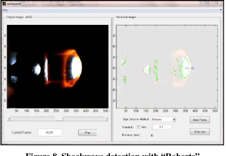
To detect shockwave accurately and effectively, a MATLAB-based image processing software is developed. A user interface window is design to help users easily load and display shockwave image sequences, as shown in Figures 8-10. Different edge detection methods can be chosen to detect the shockwave. Edge detection thresh- olds can be specified by users or automatically chosen by the program. Users can select to display random frame or play the image sequence continuously. In either case, the edge detection results will be displayed at the same time.
quence #1, all methods measure the shockwave thickness as 10 pixels; while for sequence #2, all methods agree that the shockwave thickness is 9 pixels. Users can select edge detection method according to their applications or the characteristics of the image sequence. For example, if the sequence has a higher level of noise, then “Canny” or “LoG” can be used due to their noise resistance property. However, these two methods have higher computational complexities. For quick detection applications, the other three methods may be more suitable.
Figure 8. Shockwave detection with “Roberts”.
[image:5.595.57.296.214.713.2]Figure 9. Shockwave detection with “Sobel”.
Figure 10. Shockwave detection with “Canny”.
Table 1. Shockwave thickness detection results.
Shockwave Thickness (pixels) Edge Detection Method
Sequence #1 Sequence #2
Roberts 10 9
Prewitt 10 9
Sobel 10 9
Canny 10 9
Laplacian of Gaussian 10 9
a. All edge detection methods choose thresholds automatically.
5. Conclusions, Challenges, and Future
Works
A shockwave detection system is built. The system util- izes image edge detection algorithms to easily and accu- rately detect shockwave. Based on the experimental re- sults, the system meets the design requirements. How- ever, there exists some challenges. The biggest challenge right now is how to deal with the large volume of data captured by high speed camera as well as the high com- putational complex image processing algorithms. To load the whole sequence in computer, 8 GB main memory is required. To accomplish real time processing, high-per- formance computer system is desired. The future works include testing this software system on the HPC system make the system more user friendly.
6. Acknowledgements
This work was partially supported by the NSF SEED award.
REFERENCES
[1] L. G. Roberts, “Machine Perception of Three-Dimensiona l Solids,” Optical and Electro-Optical Information
Proc-essing, J. T. Tippett, et al., Eds., May 1965.
http://www.packet.cc/files/mach-per-3D-solids.html#*
[2] J. M. S. Prewitt, “Object enhancement and extraction,”
Picture Processing and Psychopictorics, B. Lipkin and A. Rosenfeld, Eds., New York: Academic Press, 1970, pp. 75-149.
[3] I. E. Sobel, “Camera Models and Machine Perception,” Stanford Doctoral Dissertation, 1970.
[4] J. Canny, “A Computational Approach to Edge Detec-tion,” IEEE Transactions on Pattern Analysis and
Ma-chine Intelligence, Vol. PAMI-8, No. 6, 1986, pp.
679-698.doi:10.1109/TPAMI.1986.4767851
[5] D. C. Marr and E. Hildreth, “Theory of Edge Detection,” in Proceedings of the Royal Society of London, Vol. 207, No. 1167, Feb. 1980, pp. 187-217.
[image:5.595.56.287.217.377.2]