Exploring Greek innovation activities: the adoption of generalized linear models

Munich Personal RePEc Archive

Exploring Greek innovation activities:

the adoption of generalized linear models

Halkos, George

University of Thessaly, Department of Economics

2010

Online at

https://mpra.ub.uni-muenchen.de/24392/

Exploring Greek Innovation activities:

The adoption of Generalized Linear Models

George Halkos

1

and Christos Kitsos

2

1

Department of Economics, University of Thessaly

2

Technological Educational Institute of Athens

Abstract

In this paper we examine the innovative performance of Greek firms in terms of the women participation in research and technological development. For this reason we rely on the final results of a research project on women in innovation, technology and science, based on 279 questionnaires selected on a two years time period (2004-2006). Concerning the female participation in innovations a number of variables are used, like the total number of women employees by age, by education level, by firm size and by sector, as well as women in product and in process innovations, their position in the firm (owner, manager) and finally equality in job enrichment, in salary, in education– training and in promotion. Apart of presenting the empirical results relying on the analysis of the data collected by the survey to the Greek enterprises, we use the collecting variables in an econometric formulation using logistic regression and extracting the associated probabilities for implementing innovations. For this reason, first the General Linear Model (GLIM) is introduced and statistical inference and estimation problems are discussed. Then the Logit Model is presented under the theoretical framework of the Generalized Linear Models (GLIM), while some theoretical inside is extended with a number of suggested propositions and theorems.

Keywords: Innovation, Entrepreneurship, Competitiveness, Diversity.

JEL Codes: O31, Q55, L26, C10

Address for Correspondence

George Emm. Halkos

Director of Postgraduate Studies

Associate Editor in Environment and Development Economics Director of the Operations Research Laboratory

Deputy Head

Department of Economics University of Thessaly Korai 43

Volos 38333, Greece

Τel. 0030 24210 74920

Introduction

Innovation refers to a new or significantly improved product (good or service) introduced to the market. Innovations rely on the results of new technological developments, new combinations of existing technologies and production methods or the utilisation of other knowledge acquired by the firm during its operation. Specifically product innovation may take place with respect to its fundamental characteristics, its technical specifications, potential uses, or user friendliness. Innovation may also refer to the introduction within a firm of a new or significantly improved process. A process innovation includes new and substantially improved production technology, better and easier methods of supplying services and of delivering products. Innovations may be developed either by the innovating firm or by another firm. Innovations should be new to the firm under consideration. For product innovations they do not necessarily have to be new to the market and for process innovations the firm does not necessarily have to be the first to have introduced the process.

The emphasis in the existing literature is mainly on an increasing relevance of knowledge and innovation as an input to production and innovative processes (OECD, 2001). The OECD (1996) report on ‘The Knowledge-based Economy’ clarifies the terms used in describing the ‘New Economy’. The increasing contribution of high-tech sectors (computers, electronics and aerospace) to GNP and employment as well as the recognition of the role of knowledge and technology in economic growth has led to the establishment of the term ‘knowledge-based economy’ (OECD 1996, p. 9).

In innovation management, the first explicit theory is the “technology push theory or engineering theory of innovation”, where basic research and industrial R&D are the sources of new or improved products and processes. The production and uptake of research follows a linear sequence from the research to the definition of a product and specifications of production. Alternatively and in the 1960s, the “market pull theory of innovation” gave a central role to research as a source of knowledge to develop or improve products and processes.

The latter theory recognizes for the first time the organisational factors as contributors in innovation theory. Technical feasibility was still considered as necessary condition for innovation but no longer sufficient for successful innovation (Schmookler, 1996; Myers and Marquis, 1969). Here is where a new generation called the “chain-link theories” of innovation emerged in order to explain that linkages between knowledge and market are not as automatic as assumed in the technology push and the market pull theories of innovation (Von Hippel, 1994).

At the end of the 1980s and during the 1990s, a technological networks theory of innovation management was developed by a new group of experts as “systems of innovation”. According to Nelson (1993) and OECD (1999) this view emphasizes the significance of external to the firm information sources such as clients, suppliers, consultants, government laboratories and agencies etc. Finally, “the social network theory” of innovation management may be considered which states that knowledge is crucial in facilitating innovation. According to Foray (2000) the increasing and steadily growing significance of knowledge as a production factor and as a determinant of innovation is explained by the continuous accumulation of technical knowledge through time, as well as by the use of communications technologies that facilitates this knowledge making it available instantly worldwide.

provide the theoretical background of the adopted Generalized Lineal Model theory, so crucial in any Risk Analysis problem and we also extensively discuss the Greek case of female participation in innovation activities of firms. We are relying on the results of a research project on women in innovation, technology and science, based on 279 questionnaires selected on a two years time period (2004-2006), when 2200 questionnaires were delivered across the country, to firms with more than 20 employees. In this paper cconcerning the female participation in innovations a number of variables are used. Specifically, the total number of women employees by age, by education level, by firm size and by sector, as well as women in product and in process innovations, their position in the firm (owner, manager) and finally equality in job enrichment, in salary, in education–training and in promotion.

Apart of presenting the empirical results relying on the analysis of the data collected by the survey to the Greek enterprises, we use the collected variables in an econometric formulation using logistic regression and extracting the associated probabilities for implementing innovations. For this reason, first the General Linear Model (GLIM) is introduced and statistical inference and estimation problems are discussed. Then the Logit Model is presented under the theoretical framework of the Generalized Linear Models (GLIM), while some theoretical inside is extended.

The structure of the paper is the following. Section 1 introduces the theoretical background of the GLIM while section 2 discusses the logistic model as a special case of GLIM. Section 3 presents an empirical application in the case of innovation activities in Greece. In particular this section discusses the data used, the basic descriptive empirical findings and the results derived using a logistic regression formulation. The final section concludes the paper.

1. Generalized Linear Models (GLIM)

1.1Linear Models

Models of the general form

y=Xβ+e (1.1.1)

where y is a n x 1 vector of responses, β is a p x 1 vector of parameters, X is a n x p

matrix with elements zeros or ones or values of the so-called “independent” or “input” or “explanatory” variables and e is an unobserved n x 1 vector of errors attracted

interest the 20th century. There is an extended bibliography in English and in Greek,

see Halkos (2006), Kitsos (2006) among others. All the theory of Linear Models (or General Linear Model – GLIM) is based on the hypothesis that the errors are

independent and identically distributed with normal distribution N(0,σ²).

But it has been noticed that the responses, y, might have distribution other than the Normal or might be categorical rather than continuous. And even more the “link”

between the responses y and the explanatory variables, with form the matrix X, might

not be linear of the form (1.1.1). Although these are disadvantages there are some advantages to keep the theoretical balance:

1. Many of the properties of the Normal distribution can be faced to a wider class

2. There are numerical extensions from the estimation of the form Xb to the general form g(Xb) (see section 2)

These two main points provided evidence for the development of the Generalized Linear Models theory, covering the General Linear Models.

1.2 Exponential family of distributions

Consider a single random variable Y whose probability function is either discrete or continuous. We shall say that it belongs to the exponential family if the probability function can be written as

f(y;θ) = γ(y) t(θ) ea(y)b(θ) (1.2.1)

where a(.), b(.), γ(.), t(.) are known functions, θ∈Θ ⊆_฀ p

is the vector of unknown

parameter from the parameter space Θ ⊆฀ p. In practice usually p=2, that is only two

parameters have to be estimated. In most theoretical approaches Θ is assumed compact

so that if there are any sequences assumed (as in sequential analysis problems) the

sequences converge within Θ.

The (1.2.1) form can be reduced to

f(y;θ)=exp{a(y)b(θ)+C(θ)+d(y)} (1.2.2)

where γ(y)=ed y( ), t(θ)=exp[C(θ)].

If γ(y)=y the (1.2.2) is known as the canonical form. The term b(θ) is known also as the

natural parameter of the distribution. If there are additional parameters, besides θ, they

are acting as “nuisance parameters” forming part of a, b, c, d and they are assumed to

be known (although might not be!)

For the well-known distributions Poisson, P0(λ), the normal N(μ, σ²) and the binomial

B(n; y, p) which belong to the exponential family. Table 1 below summarizes the mentioned terminology.

Table 1: Poisson (λ), Normal N(μ, σ²), Binomial(n; y, P) from the exponential family

Distribution Natural parameter C d

P0(λ) Logλ -λ -logy!

N(μ, σ²)

2 μ σ

2

2 2

1

log 2 2

μ _πσ

σ

⎡ ⎤

− _⎢ + _⎥

⎣ ⎦

2

2

1 2

y

σ −

B(n; y, P)

log 1

P P

−

(

)

log 1 n −P

log n

y

⎛ ⎞ ⎜ ⎟ ⎝ ⎠

Notice that from (1.2.2) the likelihood function L (the joint distribution function for the

1 1 1

( ; ) exp ( ) ( ) ( ) ( )

n n n

i i i

i i

i

L f y θ bθ a y nGθ d y

= =

=

⎧ ⎫

= = _⎨ + + _⎬

⎩

∑

∑

⎭

∏

(1.2.3)

The statisticT =

∑

a y( )_i is called sufficient statistic for b(θ). Practically this means that

the statistic T, the summation, summarizes all the information about θ.

Now, the target is to find “closed”, if possible, expressions for the expected value and variance, so that inference to be feasible for a(y). The main implication is the so called Granger-Rao theorem (see Kitsos and Edler, 1997) and for a theoretical framework Scherrish (1995). Let us now discuss how this can be useful in practical problems.

Consider the log-likelihood l and U l

θ ∂ =

∂ ,

2 '

2

l U

θ ∂ =

∂ . Then it can be proved that

( ) 0,

E U = Var U( )=E U( 2)−E(−U') (1.2.4)

Function U is known as “score function” and the variance of U is a case of what is

called in Statistics (Fisher's) information. There are different measures of information, like Fisher's, Shannon's etc. and there are some relations among them, but this is beyond the task of this paper. Moreover we would like to emphasize that the closed forms we are looking for, do not provide solutions and therefore an old (and secure) iterative scheme is adopted: Newton-Raphson.

Here we comment that these methods are rich in theoretical background and mathematical application. So the experimentalists, and not only, were wondering how useful are really. Now with the statistical packages the results are easy to be obtained, but to interpret them, the theoretical insight is necessary. That is what we provide, in a compact form, in this section.

Consider the exponential family as in (1.2.2). The log-likelihood is

l = log f(y;θ)=a(y)b(θ)+c(θ)+d(y) (1.2.5)

Therefore we easily evaluate the score function and its derivative:

U= a(y)b'( )+c'( ), θ θ U’= a(y)b’’(θ)+c’’(θ) (1.2.6)

As E(U)=0 then

0 = E[a(y)]b’(θ)+c’(θ) ⇒ E[a(y)]= '( )

'( )

c b

θ θ

− (1.2.7)

Thus a closed form for E[α(y)] has been evaluated. Moreover, consider (1.2.4), it is

Var(U)=[b’(θ)] ² Var [a(y)]

Thus

[

]

2

[

]

2

1

( ) ''( ) '( ) ''( ) '( )

[ '( )]

'( ) '( )

1

''( ) ''( )

[ '( )]

Var a y b c c b

b

c b

c b

b

θ θ θ θ

θ

θ θ

θ θ

θ

= −

=

(1.2.8)

Therefore with (1.2.7) and (1.2.8) closed forms for the expected value and variance of

a(y), from the exponential family of models, have been evaluated.

1.3 Definition of GLIM

Nedler and Wedderburn (1972) in their pioneering paper noticed the unity a class of statistical methods, involving linear combinations of parameters. The idea of a generalized linear model came into light. We briefly follow it.

Consider Y1,Y2,...Yn independent random variables, each with a distribution form the (1.2.1) exponential family. Moreover:

i. Each of the observations Yi, i=1,2,...n has distribution of the canonical form i.e.

a(y)=y. Depending on a single θi (1.2.2) is reduced to

f(yi;θi)=exp{yib(θi)+C(θi)+d(yi)} (1.3.1)

Notice that not all θi's have to be the same

ii. The joint probability density function of Y1,Y2,...Yn is then evaluated as

1 2 1 2

1

( , ,..., ; , ,..., ) exp [ ( ) ( ) ( )]

n

n n i i i i i

i

f y y y θ θ θ y b θ C θ d y

=

⎧ ⎫

= _⎨ + + _⎬

⎩

∑

⎭ (1.3.2)

iii. We consider a “small” set of parameters β β₁, ₂,...,β_p say p<n and a (monotone

differentiable) function g, known as link function which relates the expected

value of Y E Y_i,

( )

_i =μ_L, with a linear combination of β's, i.e.

( )

T L L

g μ =X β (1.3.3)

with β =

(

β β₁, ₂,...,β_p

)

T,X_i and a p x 1 vector of explanatory variables.

Example 1: The general linear model of the form (1.1.1) y=Xβ+e is, trivially, a

GLIM model with link function

( )

T

i i i

g μ =μ =X β, i.e. the identity and

(

2

)

,

i L

Y ฀ N μ σ .

Example 2: For the binary responses Y1,Y2,...Yn, with (P Yi = = = −1) Pi 1 P Y( i =0).

The probability function of Yi is yL(1 )1 yL,

i L i

belongs to (1.2.1) family, and the link function

( )

log ,

( )

1

i

i i i

i

P

g P P E Y

P

= =

− is known

as logit function. See Section 2 for a further development. If we assume

( )

exp

( )

_{( )}

1 exp

T T

T

g p β p β

β

= ⇒ =

+ x x

x

The logit model is discussed in Section 2.

1.4 Estimation and inference for GLIM

Recall (1.2.2) and the likelihood (1.2.3). For the GLIM discussed above the log-likelihood, from (1.2.3) is reduced to

1

( ; ) ( ) ( ) ( )

n

i i i

i

l θ y y b iθ C θ d y

=

=

∑

+

∑

+

∑

(1.4.1)

and from (1.2.7) ( ) '( )

'( )

l l l

l

c E y

b

θ μ

θ

= = − (1.4.2)

The link function is g(μ_l)=xT_lβ =n_l (1.4.3)

The solution of the equation l 0

θ ∂ ₌

∂ is equivalent to the solution of 0

l

β ∂ ₌

∂ (see Cox

and Hinkely 1974, chapter 9 for details).

Therefore, under the regularity conditions, assumed for the evaluation of MLE, the evaluation of MLE seems to be an easy story. This is not the case. The MLE can be evaluated only adopting numerical methods, the most well known being the Newton-Raphson. The theoretical insight of such a choice is beyond the target of this paper. However other choices have theoretical implementation. Following Kitsos and Edler (1997) we choose a “large” set where the solution possibly lies, adopting bisection method for 2 or 3 steps and getting an initial guess in the neighbourhood of the solution. The Newton-Raphson method can be applied and convergence is “fast” with no theoretical implementations.

For (1.4.1) the following can be proved.

Proposition 1.4.1. For the log-likelihood (1.4.1) the score function can be evaluated as

1

( )

( )

n

i i ij

i i

i

i

j i i

y x

l U

Var Y n

μ μ

β =

− ⎛ ⎞

∂ ∂

= = _{⎜ ⎟}

2 2 1 ( ) ( ) ( ) T jk j k n

ij ik i jk

i i i

l

E E

x x

Var Y n

β β μ = ⎛ _∂ ⎞ = = = − ⎜_⎜ ⎟_⎟ ∂ ∂ ⎝ ⎠ ⎛∂ ⎞ = _{⎜ ⎟} ∂ ⎝ ⎠

∑

I UU I

I

Proposition 1.4.2. The Fisher's information matrix equals

(1.4.5)

Notice that Fisher's information is written as

T

=

I X WX (1.4.6)

With 2 1 ( ) i i i diag

Var Y n

μ ⎧ _{⎛∂ ⎞} ⎫ ⎪ ⎪ = _{⎨ ⎜ ⎟ ⎬} ∂ ⎝ ⎠ ⎪ ⎪ ⎩ ⎭

W (1.4.6a)

To solve the equation U l 0

β ∂

= =

∂ (1.4.7)

the Newton-Ramphson iterative scheme of the following form is adopted

1

1

U

U ν

ν ν ν

β β β β β − + = ⎛∂ ⎞ = _{− ⎜ ⎟} ∂

⎝ ⎠ (1.4.8)

But, considering the following steps with E being the “expectation”

2 2

lk

l k l k l k l k

U l l l l l l

E E

β β β β β β β β β

⎧ ⎫ ⎡ ⎤

∂ ₌ ∂ ₌ ∂ ∂ ∂ ∂ _{= −} ∂

⎨ ⎬ ⎢ ⎥

∂ ∂ ∂ ∂ ∂ ฀ _⎩∂ ∂ _⎭ I ฀ _⎣∂ ∂ _⎦(Fisher’s Information)

Therefore (1.4.8) is reduced to 1

1 U

ν ν ν ν

β β −

+ = +I (1.4.9)

The Fisher's information matrix is evaluated at β=β_ν and actually is replaced by its

estimate. Multiplying both sides of (1.4.9) by Iv we get

1 U

ν νβ + = ν νβ + ν

I I (1.4.10)

Recall (1.4.6) and notation (1.4.6a) and introduce the notation

(

)

i lk k i i

i

n

Z x β y μ

μ

∂

= + −

∂

∑

(1.4.11)

with β_κ at ν-iteration then (1.4.10) is reduced to

T T

v Z

b =

X WX X W (1.4.12)

Proposition 1.4.3 The MLE for GLIM is obtained by WLS.

As it is known in GLIM the MLE and OLS coincide. Therefore Proposition 1.4.3 is the equivalent of this result.

As far as statistical inference is concerned we note that the score function U has the multivariate normal N(0,I), therefore

1 2

T

p

χ

−

U I U฀ (1.4.13)

with I being Fisher's information matrix. The chi-square distribution plays a central role

to the GLIM theory (see expressions (1.4.18), (1.4.19) below).

Now, if we expand the score function for the parameter β around b, by Taylor

expansion then

( ) ( ) ( )( )

U β =U b +H b β−b (1.4.14)

with H(b) being the Hessian matrix, i.e. the matrix of second derivatives of

log-likelihood at β=b. Then it can be proved that

( T) ( )

E UU E H

= = −

I (1.4.15)

The following statistic (actually the “Euclidean” distance of b from β, that is how “far”

is the estimate from the true parameter)

2

( )T ( )

p

b−β I b−β ฀ χ (1.4.16)

is known as the Wald statistic. In practice is used to make statistical inference about β.

The adequacy of the model is assessed by the likelihood ratio statistic λ which equals to

( ; )

( ; )

MLE

L b y

L b y

λ = (1.4.17)

where bMLE the MLE of β, L

( )

฀ the likelihood function. Therefore λ offers a measure

of goodness of fit as the ratio of the maximal model and the model of interest. Moreover

logλ=l(b_MLE; )y −l( ; )b y (1.4.17a)

Nedler and Wedderburn (1972) defined the deviance D as

[

]

2

2 log 2 ( _MLE; ) ( ; ) _{n p}

D= λ= l b y −l b y ฀ χ ₋ (1.4.18)

[

] [

]

[

]

0 1 0 1

2

1 0

2 ( ; ) ( ; ) 2 ( ; ) ( ; )

2 ( ; ) ( ; )

MLE MLE

p q

D D D b y b y b y b y

b y b y χ ₋

= − = − − −

= −

l l l l

l l ฀

If the model is poor D will be larger predicted byχ_{n p}2₋ . Theoretical D follows a

non-central χ2, but this is beyond this paper. Thus if a model –with p parameters–

provides a good description of the collected n observation so that 2

n p

D฀ χ ₋ , we expect

D฀ N−P (1.4.18a)

The deviance D can be a helpful tool for a hypothesis testing. Indeed if we are

interesting in testing H₀:β β= ₀ vs. H₁:β β≠ ₁

with β₀ =

(

β₁,...,β_q

)

T,β₁=

(

β₁,...,p_p

)

T, 2<p<n

Proposition 1.4.4. We can test H₀ versusH₁ by adopting the difference of deviances under H₀ andH sayD D₁, ₀, ₁ respectively.

Indeed:

(1.4.19)

Thus if D has been evaluated greater than the upper tail 100% point of the 2

p q

χ ₋ we

reject H0 in favour of H1 – i.e. even though β1 has too many parameters does not fit the

collected data set satisfactory. Notice that F distribution can be used only for model involving normal distribution. In such a case

0 1 1

,

p q n p

D D D

F F

p q n p − −

− =

− − ฀ (1.4.20)

If H₀ is not correct the calculated value of F will be larger than the value of the

corresponding F_{p q n p− , −} distribution, at the predefined level.

2. Logistic Regression

The logistic regression is a particular case of a GLIM. We are going to discuss the simple logistic model next.

2.1 Introduction

Let us formulate the problem. We are working with generalized linear models (GLIM), were the response is a binary variable declaring “success” or “failure” as was above discuss. Let W be such a variable:

1 if the outcome is success

0 if the outcome is failure (2.1.1)

With P W

(

= = = −1

)

π 1 P W

(

=0

)

(2.1.2)

Certainly any number could declare success or failure say -1 and 1, 5 and 15 BUT we are using 1 and 0 (and the statistical packagers only these values realize) as we are NOT interested in W eventually, but on the summation of values W.

Actually if they are observed in such independent random variables with assessing probability then the joint probability is evaluated as.

(

)

1

1 1

1

(1 ) exp log log 1

1

i i

n n n

w w i

i i i

i i

i i

w π

π π π

π

−

= =

=

⎧ ⎛ ⎞ ⎫

⎪ ⎪

− = _{⎨ ⎜ ⎟}+ − _⎬

−

⎪ ⎝ ⎠ ⎪

⎩

∑

∑

⎭

∏

(2.1.3)

Notice that (2.1.3) belongs to the exponential family of models discussed in section (1.2) assuming that πi’s are equal, i.e.

1, success with probability π

0, failure with probability 1-π (2.1.4)

In such a case if we define the random variable as

1

n i i

Y w

=

=

∑

=number of successes (2.1.5)

it is a binomial distribution with probability density function defined as

( ) n y(1 )n y

P Y y

y π π

−

⎛ ⎞ = =_{⎜ ⎟} −

⎝ ⎠ y = 0, 1, …, n (2.1.6)

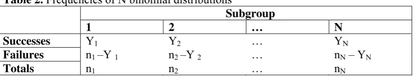
So we can classify the data as in Table 2 if N independent random variables Y1,Y2,...YN

[image:12.595.87.516.668.747.2]

corresponding to the number of successes/failures are assumed.

Table 2. Frequencies of N binomial distributions

Subgroup

1 2 … N

Successes Y1 Y2 … YN

Failures n1 –Y 1 n2 –Y 2 … nN – YN

Totals n1 n2 … nN

W =

The most typical case in practice is to consider two subgroups. Examples are employment/unemployment for men/women, getting or not a characteristic for patient /not patient, etc.

2.2 Generalized Linear Models

The target is to ”describe”, to “analyze” the proportion of successes i

i i

Y P

n

= , in

each subgroup (see Table 2.1) in terms of e.g. factor levels, sex age etc acting as

explanatory variables Xi which “describe” the subgroup. That is we are interested in

assuming that there is a link function which is modelling the probabilities πi as

( )

T i i

g π =X β (2.2.1)

with β being a vector of parameters.

Trivially if g

( )

π_i =XT_iβ then π =g−1

(

XTβ

)

and as π needs to be within [0,1] we assume the existence of a cumulative distribution function (cdf) F such that

( )

( )

1

( )

t

T

g

F t

f w dw

π

−

β

−∞

=

x

=

=

∫

(2.2.2)

as by the definition of the cdf a distribution function f exists such that (2.2.2) to be true. This probability density function f(w) is called tolerance distribution. As there are various tolerance distributions we shall focus our attention on

( )

[

1 0 1

]

2

0 1

exp( )

1 exp( )

w f w

w

β β β

β β

+ =

+ + (2.2.3)

known as logit or logistic model. From (2.2.3) and (2.2.2) we have

( )

0 1

0 1

exp( )

1 exp( )

x x

f w dw

x

β β

π

β β

−∞

+

= =

+ +

∫

(2.2.4)

Therefore the link function (see (2.2.1)) is

( )

log 0 1

1

g π π β β x

π

= = +

− (2.2.4α)

This link function, log 1

π π

− ,is known as logit function or logit transformation.

2.3 MLE for the Logit

0 1 1

0 1 1

exp( )

1 exp( )

i x x β β π β β + = + +

So log _{0 1} log 1

(

)

log 1 exp

(

_{0 1}

)

1

i

i i i

i

x x

π _{β β π β β}

π = + ⇒ − = − ⎡⎣ + + ⎤⎦

− (2.3.1)

From (2.1.3) and (2.3.1) we get the log-likelihood function equal to

(

0 1

)

(

0 1

)

1

log 1 exp log

n

i

i i i i

i i

n

y x n x

y

β β β β

= ⎧ ⎛ ⎞⎫ ⎪ ⎪ = _⎨ + − ⎡_⎣ + + ⎤_⎦+ _{⎜ ⎟⎬} ⎪ ⎝ ⎠⎪ ⎩ ⎭

∑

l (2.3.2)

Therefore the score functions with respect to β0 and β1 are evaluated as

(

)

(

)

0 1 0 1 1 1 n

i i i i

n

i i i i i

U y n

U x y n

π β π β = = ∂ = = − ∂ ∂ = = − ∂

∑

∑

l

l (2.3.3)

Therefore Fisher's 2x2 information matrixIis evaluated equal to

(

)

(

)

(

)

2

(

)

1 1

1 1

i i i i i i i i i i i i i i

n n x

n x n x

π π π

π π π π

⎛ − − ⎞

= ⎜_{⎜ − −} ⎟_⎟

⎝ ⎠

∑

∑

∑

∑

I (2.3.4)

Recall that MLE are obtained through the iterative scheme

1 1 1 U 1

ν−βν = ν−βν− + ν−

I I (2.3.5)

see (1.4.10). Therefore an initial guess should be provided. To “feed” (2.3.5) initial

guesses might be used - take β_0,0 =0, β_1,0 =0. The estimated variance-covariance

matrix is⎡_⎣I

( )

β_ν ⎤_⎦−1, the fitted values then are ˆy_i =n_iπˆ_i and

• the log-likelihood ratio statistic is

(

)

1

log log log

ˆ ˆ

n

i i

i i i

i i i

y n y

y n y

y n y

λ = ⎡ ⎛ ⎞ ⎛ − ⎞⎤ = _{⎢ ⎜ ⎟}+ − _{⎜ ⎟⎥} − ⎝ ⎠ ⎝ ⎠ ⎣ ⎦

∑

(2.3.6)

As 2 logD= λ see (1.4.18) and ˆy_i =n_iπˆ_i we get from (2.3.6) that the deviance D is

(

)

1

2 log log

ˆ ˆ

n

i i

i i i

i i i i

y n y

D y n y

nπ n nπ

= ⎡ ⎛ ⎞ ⎛ − ⎞⎤ = _{⎢ ⎜ ⎟}+ − _{⎜ ⎟⎥} − ⎝ ⎠ ⎝ ⎠ ⎣ ⎦

Notice that (2.3.6a) does not involve any nuisance parameters and recall that D฀ χ_{n p}2₋ , see (1.4.18a).

2.4 Goodness of fit

Recall that Pearson'sχ2

statistic is defined as

(

)

2

2 O E

E

χ =

∑

− (2.4.1)

That is (2.4.1) offers a measure of distance between the observed (O) and the expected values (E). For the cells of Table 2.1 this is clear.

For the model under investigation

( )

i i i

E Y =nπ and Var Y

( )

_i =n_iπ_i

(

1−π_i

)

• so the weighed sum of squares

(

)

(

)

2

2

1 1

n

i i i _{i i i}

y n

WSS

n

π

π π

=

− =

−

∑

(2.4.2)

has a meaning to attract interest.

Proposition 2.4.1 The WSS is equivalent toχ2. Indeed, if we consider (2.4.1):

(2.4.3)

Therefore when is calculated at the estimated values is

(

)

(

)

2 2

1

ˆ

ˆ 1 ˆ

n

i i i cal

i i i i

y n

n

π χ

π π

=

− =

−

∑

(2.4.4)

A very nice result for theχ2, measure of distance between observed and expected

values is that

Proposition 2.4.2 Relation (2.3.6) is equivalent to (2.4.4). Therefore the evaluated

deviance for the logit model coincided with the calculated χ_cal2 values.

Indeed:

(

)

(

)

(

)

(

)

(

)

(

) (

)

2 2

2

1 1

2

1

1

1

1 1

n n

i i i i i i i

i i i i i i

n

i i i

i i i i i i

n y n y n

n n

y n

WSS n

π π

χ

π π

π

π π

π π

= =

=

− − −

⎡ ⎤

− _{⎣ ⎦}

= +

− −

= − + =

−

∑

∑

(

)

(

)

(

)

(

) (

)

(

) (

)

(

)

1 2 1 2 2 1 2

2 log log

ˆ ˆ ˆ 1 ˆ 2 ... ˆ 2 ˆ 1 ˆ 2 ... ˆ 2 ˆ ˆ n i i i

i i i

i i i i i i

n

i i i i i i

i i i

n _{i i i i i}

i i i i i

i i i i

i i i i

n y y

D y n y

n n n

y n y n

n

n y n n

n y n n

n n y n n π π π π π π π π π π = = = ⎡ ⎛ ⎞ ⎛ + ⎞⎤ = _{⎢ ⎜ ⎟}+ − _{⎜ ⎟⎥} − ⎝ ⎠ ⎝ ⎠ ⎣ ⎦ ⎡ ₋ ⎤ − + + + ⎢ ⎥ ⎢ ⎥ ⎣ ⎦ ⎡⎧ _{⎡ − − − ⎤} ⎫⎤ ⎢⎪ ⎣ ⎦ ⎪⎥ + _⎢⎨⎡_⎣ − − − ⎤_⎦+ + _⎬⎥ − ⎪ ⎪ ⎢_{⎩ ⎭}⎥ ⎣ ⎦ −

∑

∑

∑

l ฀ ฀

(

)

2

1 1 ˆ

n

cal i i i

χ π = = −

∑

We shall apply the Taylor series expansion of KlogK

L about K=L, of the form

(

)

1

(

)

2

log ...

2

K L

K

K K L

L L

−

= − + +

We apply this Taylor expansion for the two terms of D with K =Y_i,L=nπˆ_i and

( _{i i})

K = n −y and L= −n_i n_iπˆ_i as follows

(2.4.5)

2.5 Extensions

Let us now discuss another very important index in Logistic analysis, the odds

ratio. First we define the distributional properties of the dependent variable1, which

is a dichotomous variable Y taking the value of 1 with probability Θ and the value of

0 with probability 1-Θ. Such a random variable has a simple discrete probability

distribution given as

Pr (Yi , Θi ) = i i

Y i Y i − Θ − Θ 1 ) 1

( (2.5.1)

Given the mutually independent Y1, Y2,…,Yn, the likelihood function of (2.5.1) is the

product of the marginal distributions for the Yi ’s. Specifically

L(Y;Θ)= Pr( ;Y_{i i})

(

_iY

(

_i

)

Y

)

i n

i n

i i

Θ = Θ −Θ −

=

=

∏

∏

1 1

1 1

(2.5.2)

where Θ=(Θ1 , Θ2, …, Θn).

In our sample the first n1 out of n observations have the characteristic under

investigation (employment – unemployment, having information – not having

1

information etc) and so Y1=Y2=…=Yn₁=1 while the rest of the observations do not and

so

1 1

n

Y ₊ =

1 2

n

Y ₊ =…=Yn=0. This means that expression (2.5.2) becomes

L(Y;Θ)=

1 1 1 1 (1 ) n n i i

i= i n= +

⎡ ⎤

⎛ ⎞

Θ _⎢ − Θ _⎥

⎜ ⎟

⎝

∏

⎠ ⎣

∏

⎦ (2.5.3)

If Xi =(Xi1, Xi2, …,Xik) the set of values of the k independent variables X1, X2, …, Xk

specific to individual i then the logistic model assumes that between Θi and Xij’s a

specific form exists which is given by

0 1 1 1 exp k j ij j i X β β = ⎡ ⎛ ⎞⎤ ⎢−⎜ + ⎟⎥ ⎜ ⎟ ⎢ _{⎝ ⎠}⎥ ⎣ ⎦ Θ = ∑ +

i=1,2, …, n (2.5.4)

Obviously βj are unknown coefficients to be estimated by regression. Replacing Θi in

(3) we derive the likelihood function as

L(Y;β) =

1 0 1 0 1 ( ) 1 1 exp 1 exp k ij j k j ij j n X i X n i β β β = = + = ⎛ ⎞ ⎜ + ⎟ ⎜ ⎟ ⎝ ⎠ = ∑ ⎡ _∑ ⎤ ⎢ ₊ ⎥ ⎢ ⎥ ⎢ ⎥ ⎣ ⎦

∏

∏

(2.5.5)

Although we assume an unconditional maximum likelihood function that could lead to

biased estimates of β’s as our data size is large this potential problem is not so serious.

The regression coefficients β’s of the proposed logistic model quantifies the

relationship of the independent variables to the dependent variable involving the

parameter called the Odds Ratio (OR).

Definition 2.5.1. As odds we define the ratio of the probability that implementation will take place divided by the probability that implementation will not take place.

That is Odds (E⏐X1, X2, …, Xn) =

Pr( ) Pr( )

E E

1− (2.5.6)

Instead of minimizing the squared deviations as in a multiple regression, logistic regression maximizes the likelihood that an event will take place.

0 1 1 2 2

Pr( )

ln ...

1 Pr( ) k k

E

X X X

E =β +β +β + +β

− (2.5.7)

or Pr(E)

where P is the probability of having the characteristic under investigation given the independent variables X1, X2,…, Xk. Equation (2.5.8) models the log of the odds as a linear function of the independent variables and it is equivalent to a multiple regression equation with log of the odds as the dependent variable.

The logit form of the model is a transformation of the probability Pr(Y=1) that is defined as the natural log odds of the event E(Y=1). That is

logit [Pr(Y=1)]=ln[odds (Y=1)]=ln Pr( )

Pr( )

Y Y

=

− =

⎡ ⎣

⎢₁ 1₁ ⎤_⎦⎥ (2.5.9)

Let us consider the general case, where the dichotomous response variable Y, denotes whether (Y=1) or not (Y=0) the characteristic under investigation (employment – unemployment, having information – not having information etc) is linked with the k regression variables X=(X1, X2, …., Xk) via the logit equation

0 1

0 1

exp

( 1)

1 exp

K k k k

K k k k

X P Y

X

β β

β β

= =

⎧ ₊ ⎫

⎨ ⎬

⎩ ⎭

= =

⎧ ⎫

+ _⎨ + _⎬

⎩ ⎭

∑

∑

(2.5.10)

This is equivalent to

logit Pr(Y=1⎜X)= ₀

1

K k k k

X

β β

=

+

∑

With this formulation we have the benefit that the relative risk (RR) for individuals

having two different sets X′ and X of risk variables is

[

]

1

( ) 1 ( )

exp ( )

( )[1 ( )]

K

i i i i

P X P X

RR X X

P X P X = β

′ − ⎧ _′ ⎫

= = _⎨ − _⎬

′

− _⎩

∑

_⎭ (2.5.11)

It is essential that the RR of the k regressors (RRk) influences the RR of the k+1

regressors, RRk+1 as in relation (2.512) below, due to the following Theorem 2.5.1.

Theorem 2.5.1

Let the relative risk of as above in (2.5.11) is

1

K K i i

i

RR β δ

=

=

∑

with δ_i =X_i′−X_i

Then if a variable is added the relative risk of the k+1 variable equals the k-variables relative risk times the new variable relative risk, ie.

RRk+1 = RRk rk+1 (2.5.12)

Proof

1

1

1

exp

K

K i i

i

RR β δ

+ +

=

⎧ ⎫

= _{⎨ ⎬}=

⎩

∑

⎭ 1 1

1

exp

K

i i K K i

β δ β δ_{+ +}

=

⎧ ₊ ⎫₌

⎨ ⎬

⎩

∑

⎭

{

1 1

}

1

1

exp exp

K

i i K K K K

i

RR r

β δ β δ_{+ + +}

=

⎧ ⎫ _{= ⋅}

⎨ ⎬

⎩

∑

⎭

Where the definition of rK+1 is obvious. So the relative risk of the incoming K+1

variable is

1 1 K K K RR r RR + + = .

Now suppose that v is an indicator variable denoting whether or not (v=1 or v=0) someone is sampled. If we denote by

μ1 = P(v=1⏐Y=1)

μ0 = P(v=1⏐Y=0) (2.5.13)

the probability that the one with the characteristic is included in the study (μ0) and the

probability that the one without the characteristic participates as a control then the

conditional relative risk influences only the constant term β0, while the rest part of RRK

remains “invariant”, due to the following Theorem 2.5.2.

Theorem 2.5.2

The relative risk defined as the conditional probability that a person has the characteristic, given that has risk variables X and also was sampled from the

case-control studies is of the form (2.5.10) with constant term β0′ equal to:

0 1 0

0 logμ

μ β

β′ = + (2.5.14)

Proof:

From Bayes′ theorem

P(Y=1⏐v=1,X)= =

= = + = = = = = = ) / 1 ( ) , 1 / 1 ( ) / 0 ( ) , 0 / 1 ( ) / 1 ( ) , 1 / 1 ( X Y P X Y v P X y P X Y v P X v P X Y v P 1 0 1

0 1 0

1 exp exp k i i i k i i i X X

μ

β

β

μ μ

β

β

= = ⎧ ₊ ⎫ ⎨ ⎬ ⎩ ⎭ = ⎧ ⎫ + _⎨ + _⎬ ⎩ ⎭

∑

∑

_⎭⎬⎫= ⎩ ⎨ ⎧ ₊ + ⎭ ⎬ ⎫ ⎩ ⎨ ⎧ ₊ =

∑

∑

= = k i i i k i i i X X 1 0 0 1 1 0 0 1 exp 1 exp β β μ μ β β μ μ 0 1 0 1 exp 1 exp k i i i k i i i X X β β β β = = ⎧ _{′ +} ⎫ ⎨ ⎬ ⎩ ⎭ ⎧ _′ ⎫ + _⎨ + _⎬ ⎩ ⎭

∑

∑

With β₀′as in (2.5.14).

Let us now estimate the marginal influence of extra regressors. It is known that

the percentile point Lp, for the cumulative distribution function F(x) is defined as

F(Lp)=p. Therefore for the logistic Λ(⋅), say, we have

(

)

{

1

}

0 1

: 1 exp ( )

p p

L θ ⎡ θ θL ⎤− p

Λ = + _⎣− + _⎦ = (2.5.15)

Solving equation (2.5.15) for Lp it can be evaluated that

(

)

[

₀ ln 1 1

]

1

1 + −

−

= − −

p

L_p θ θ (2.5.16)

1 0 θ θ − =

M (2.5.17)

In economical analysis the median M, although a biased estimator, is sometimes, more useful than the unbiased mean, as it offers a better measure of the location of the data. Median, even under the minimax criterion, is not selected compared to the mean. But as it remains invariant if the “end-points” change drastically it is a better location measure in many cases of the economical data analysis. Consider that the value of Lp in (2.5.16) is a function of the parameter, i.e. Lp=Lp(θ), with θ=(θ0, θ1). With the above discussion in mind, we state and prove the following proposition.

Proposition 2.5.1:

The minimization of the variance of the percentile point Lp, Var(Lp), is (approximately)

equivalent to minimize the

( )

C I C F

T −1 θ

(2.5.18)

With C=(1,Lp) and 1

*

− F

I the (average per observation) Fisher’s information and θ=(θ0,

θ1).

Proof:

It is known, in principle for the exponential family of models, with response η it is

T T

F vv

I (θ)=σ−2(∇η)(∇η) = (2.5.19)

where the definition of the vector v is obvious, and vT is the transpose of v, and ∇ is the

“grand” vector asn usually. Moreover in many of the nonlinear problems the covariate u and the parameter θ appears “together” linearly, i.e. η =η(θTu). In such a case

( )

[

wθTu

]

1/2u

η =

∇ with

2

)

( _⎢⎣⎡ _⎥⎦⎤

∂ ∂ =

z z

w η , z=θTu.

That is Fisher’s information matrix is

T T F w u uu

I (θ)=σ−2 (θ ) _(2.5.20)

With σ2 the involved variance, practically a function of the unknown parameters we are

asked to estimate. Obviously the Logistic model obeys on the “intrinsic” linearity

described above. Then for the MLE of θ, θ)=(θ)₀,θ)₁)and for ni the number of

observation at ui i=1, 2 and Σni=n large, then from (2.5.20), we have

[

]

{

}

1

1

0, ) ( )1 ( )

( )

( = =

∑

Λ −Λ T _i −

i i i

i u uu n

u Var

Var θ) θ) θ) (2.5.21)

Based on the fact that I_F−1(θ)=Var(θ)and u2 =(1, u2), i=1,2. From (2.5.21) the

evaluation of Var(L)_p)equals

= ∇ ∇

=( ) ( )( ) )

( p

T p

p L Var L

L

Var θ) *

( )

1

T F

Where I_F−1(θ)=n−1

∑

I(θ), with I(θ) Fisher’s information and * 1

( )

F

I− θ the average per

observation information matrix.

2.6 Discussion on the Odds Ratio

Consider the typical scheme in logit problems

Risk Group Case Control

Characteristic XX P1 P0

Non – XX 1-P1 1-P0

The probability P1 represents the probability that a “sample case member” (e.g. patient exposed to the risk factor, unemployed attended certain seminar, company adapted an

innovation process, etc) exposed to the risk factor. The probability P0 is the probability

that a simple “control member” is exposed to the risk factor.

The odds ratio (OR) or relative risk (RR) is defined as

RR or 1 1 1 0

0 0 0 1

(1 )

/(1 )

/(1 ) (1 )

P P

P P

OR

P P P P

− −

= =

− − (2.6.1)

A χ2 test of the null hypothesis H0: OR=1 vs H1: OR≠1 is identical to a test of equality

of the two proportions, i.e.

H0: P0 =P1 vs H1: P0≠P1 (2.6.2)

The crude odds ratio can be biased due to population heterogeneity caused by confounding factors, associated with the response. Significance tests and confidence intervals for the crude OR were introduced by Mantel and Haenszel (1959) in their pioneer paper.

In the typical case where

0 1

0 1

( / )

1 exp( )

x P case x

x

β β

β β

+ =

+ + (2.6.3)

With the dichotomous variable X=1 for the high risk (characteristic – XX) and X=0 for the low-Risk (non - XX), the odds ratio is given by

OR=exp(β1)=RR≅exp(βˆ1)

underlying that the above notation was adopted.

• That is the Relative Risk (RR) or (OR) testing hypothesis H0: RR=1 is

equivalent to H0: β1=0.

When interest is focused on the trichotomous factor XX versus XY versus YY

X1=1 if XX holds

=0 otherwise

X2=1 if XY holds

=0 otherwise

Therefore YY is the reference class. The equation of the model is

Logit P(case ⏐x1, x2;z)=β0+β1 X1 +β2X2 +γZ

In such a case there are two different relative risks or odds ratios of the form

OR1=RR1=exp(β1)≈exp(βˆ₁)

OR2=RR2=exp(β2) ≈exp(βˆ₂) (2.6.4)

The OR1 provides a measure of the relative risk or odds ratio of XX versus YY, while

OR2 is a measure of OR or RR of XY versus YY, adjusted for the confounders of Z. When the variable Z is included in the logit model with one variable still the OR=exp(β1).

3. The Greek Innovation activities

In the following the Greek innovation activities are discussed through the logit model and an empirical application, due a survey we performed to the Greek firms. We explain this analysis below.

3.1 DATA

The data used in this study rely on our survey to the Greek enterprises through ‘ARCHIMEDES’ program, mentioned above. The target population of the survey is the total population of 63.000 firms, included in the database of ICAP SA (the largest Business Information and Consulting firm in Greece). The constructed questionnaire is based on Community Innovation Survey (CIS) while the methodological basis of this survey is provided by the “Oslo manual”, a joint publication of Eurostat and OECD. The selection of the sample is based on proportional stratified random sampling. The analysis focuses mainly on the small and medium-sized manufacturing enterprises and on services enterprises employing 20 or more employees. To avoid any bias resulting from response behaviour, a non-response analysis followed up.

The main statistical unit for the survey is the enterprise. In general, innovation activities and decisions usually take place at the enterprise level, which leads to the enterprise being used as the statistical unit. The following industries are included in the target population of the survey:

- manufacturing (NACE 15-37),

- electricity, gas and water supply (NACE 40-41),

- wholesale trade (NACE 51),

- transport, storage and communication (NACE 60-64),

- architectural and engineering activities (NACE 74.2),

- technical testing and analysis (NACE 74.3),

- research and development (NACE 73),

- construction (NACE 45),

- motor trade (NACE 50),

- retail trade (NACE 52),

- legal, accounting, market research, consultancy and management services (NACE 74.1),

- advertising (NACE 74.4),

- labour recruitment and provision of personnel (NACE 74.5),

- investigation hotels and restaurants (NACE 55),

- renting of machinery and equipment without an operator (NACE 71).

The time period covered by the survey was 2000-2003 inclusive. The reference period of the survey is the year 2003. Following the European classification, the size-classes used are 20-49 employees, 50-249 employees, 250 + employees.

3.2. Empirical findings

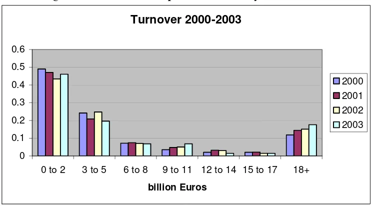
In collecting primary data, we have used a questionnaire to several sectors in Greek enterprises. The data-set was collected from 279 Greek enterprises from various sectors and several areas-prefectures of the country. From the data collected it can be seen that the R&D activities are mainly related to big firms. Also Figure 1 presents the turnover of the sampled firms and for the years 2000-2003. In the vertical axis we have the percentages while in the horizontal axis we have the turnovers in billion €.

Figure 1: Turnover of sampled firms for the years 2000-2003

Turnover 2000-2003

0 0.1 0.2 0.3 0.4 0.5 0.6

0 to 2 3 to 5 6 to 8 9 to 11 12 to 14 15 to 17 18+

billion Euros

2000 2001 2002 2003

[image:23.595.119.490.428.634.2]

They are directed towards to obtain the machinery and equipments accounting around to 58%. Education is the main source for innovation activities in Greek enterprises accounting approximately to 48% while the introduction of innovation in the market accounts to approximately 27% and the planning for production-distribution and other activities to 25 % respectively.

The following findings are based on the analysis of the collected 279

questionnaires of our sample survey (Kitsos et al., 2006). We are now at the final stage

of checking our full data set. We are proceeding our calculations on the double checked 279 responses, and we shall extent this discussion to the final data set. Our empirical results concern the total number of women employees by age intervals (namely 20-30, 31-40, 41-50, 51-60 and more than 60), women in product innovation, women in process innovation, position in firm and equality in job enrichment, in salary, in education–training and in promotion. Specifically,

- A small increase in the percentage of women in the workplace has occurred from 32% in 2000 to almost 37,5% in 2003.

- A small increase in the percentage of women graduates in the workplace has occurred from almost 33% in 2000 to almost 37% in 2003.

- Women employees between 20-30 ages (compared to 31-50 ages) are the majority of the women workforce and a small increase in the percentage has occurred from 59% in 2000 to 61% in 2003.

- The percentage of women employees is decreased as long as the age is increased to 62% for 20-30, 23% for 31-40, 10% for 41-50, 3% for 51-60 and 2% for over 60 in 2003.

- The percentage of women as Top Managers remains almost unchanged, from 21% in 2000 to 20% in 2003 while the percentage of women as Managers is increased from 33% in 2000 to 38% in 2003.

- The percentage of women employees in product innovation development is bigger (40%) than the percentage in process innovation development (33%) and the percentage of women as Top Management in product innovation development is bigger (20 %) than the percentage in process innovation development (16%). - The percentage of women as Managers in product innovation development is far

smaller (29%) than the percentage in process innovation development (45%). - The percentage of the firms with innovation activities, concerning all the four

variables of gender equality in the workplace (job enrichment, salary, training and promotion), appears to be smaller than the percentage in the total of the firms of the sample. For example, job enrichment appears to be around 37% in product innovation and 26% in process innovation comparing to 71% of the total of firms (with and without innovation activities).

According to the collected data, the main obstacles in the development of innovations are related to the lack of appropriate financial sources for innovation activities which accounts to 70% for small firms and only 10% for big firms, while the high risk activities account to about 74% for small firms and only 5% for big firms respectively. Another serious obstacle is related to the lack of information of new technologies and for the markets accounting 75% for small firms and 25% for medium firms. At the same time the lack of specialized staff accounts to 60 % for small firms and 40% for medium firms and the managerial inflexibilities account to 40 % for the small firms and 40% for the medium firms respectively.

3.3 Logit formulations and associated empirical results

As our main interest is in terms of the main effects we have ignored interactions. Only 3 and 4 out of the 12 explanatory variables were found to be statistically significant in influencing the implementation of product and process innovations respectively. Working with the most statistical significant variables we derive the logit form of the fitted model, which may be represented as

logit [Pr(Y=1)]=β0+β1Turnover+β2 PAL + β3 PFW + β4 Exp + εt

where Y denotes the dependent variable as 1 for innovations and 0 for no innovations,

the beta terms are the unknown linear coefficients needed to be estimated, and εt is the

error term, assumed from the normal distribution with mean 0 and variance 1.

Specifically the dependent variable is the answer to the question of the influence

of innovations to the products with answers ranging from high influence to no influence. The high and average influences were coded as 1 and the low and no influence as 0. The explanatory variables are Turnover taking the value of 1 for a higher than 10% increase in the turnover for the period 2000-2003 and 0 in any other

case, the PAL that is the Product Average Life which is the average life of the most

important product of the firm before it is substituted or modified. It takes the values of 1 in case of less than a year, 2 in case of 1-3 years, 3 for 4-6 years, 4 for 7-9 years, 5 in case of more than 9 years and 0 if no answer). The last significant explanatory variables are the PFW that is the percentage of female workers and Exports. The results of the fitted models are presented in Table 3.

Based on the fitted model and the information provided, it can be seen that the estimated odds ratio equals to 3,219 and 1.897 for implementing product and process innovations respectively for firms which have a higher than 10% increase in turnover, with no control for the other explanatory variables. This adjusted odds ratios of 3.219 and 1.897 mean that the odds of implementing product and process innovations is about 3.219 and 1.897 times higher respectively for a firm which has an increase of more than 10% of its turnover than for a firm which has not. The Wald statistic is statistically significant, which indicates that there is statistical evidence in these data that for firms with turnover higher than 10% the probability of implementing innovation increases.

We may compute the difference eβ$i −_{1which estimates the percentage change}

(increase or decrease) in the odds π = =

=

Pr( )

Pr( )

Y Y

1

0 for every 1 unit in Xi holding all the

other X’s fixed. The coefficient of average life of the product is β)₂=0.413, which

implies that the Relative Risk of this particular variable is β2

)

e =1.511 and the

average life of product the odds of implementing innovations increase by 51.1% ceteris paribus. In the case of process innovation the result is 1.271 implying a 27.1% increase. In relation to turnover the odds of implanting innovations increase by 221.9% and 89.7% for product and process innovations respectively keeping constant all the rest.

Similarly, the coefficient of percentage of female workers is β)₃ =-0.027 and -0.014 for

product and process innovations respectively, which implies that the Relative Risk of

this particular variable is β3

)

e =0.9733 and 0.986 and the corresponding percentage

change is eβ$2_{-1= -0.0267 and -0.014 respectively. This means that in relation to the}

percentage female workers the odds of implementing innovations decreases by almost 0.03% and 0.015 all other remaining fixed.

Table 3: Logistic Regression results

Dependent: Product Innovations Dependent: Process Innovations

Variables Estimates Odds Ratio Estimates Odds Ratio

Constant 0.483 (0.734) [0.391]

1.621

Turnover 1.169 (6.071) [0.014]

3.219 0.64

(2.895) [0.089]

1.897

PAL 0.413 (8.700) [0.003]

1.511 0.240

(4.403) [0.036]

1.271

PFW -0.027 (6.510) [0.011]

0.973 -0.014

(3.028) [0.082]

0.986

Exports 1.139

(5.252) [0.022]

3.123

Hosmer Lemeshow

8.145 [0.37]

11.135

[0.47] Likelihood

Ratio

18.121 [0.000]

28.016

[0.000] Wald statistics in parentheses and P-values in brackets.

The negative sign in the coefficient for the percentage of female workers variable requires some further thoughts. It could be explained as a higher percentage of female workers corresponding to a lower implementation of innovations. This can be considered in relation to other Departments in the firm like R&D as well as to the markets that the firm operates.

The individual statistical significance of the β estimates is presented in the column

Wald (Chi-square). The significance levels of the individual statistical tests (i.e. the P-values) are presented in the column P-value and correspond to Pr>Chi-square. Note that the variable average value of product is significant in all the usual statistical levels (0.01, 0.05 or 0.1) while the variables turnover and percentage of female workers are

statistically significant at α =0.05 and α=0.1 while the constant term is not statistical

innovations where however the variable Exports seems to have a significant influence both in magnitude as well as in statistical terms.

To assess the model fit we compare the log likelihood statistic (-2 log L$) for the

fitted model with the explanatory variables with this value that corresponds to the reduced model (the one only with intercept). The likelihood ratio statistic for comparing the two models is given by the difference

LR = -2 log L$R-(-2 log L$F)=18.121

where the subscripts R and F correspond to the Reduced and Full model respectively. The corresponding value of the test in the case of the process innovations is 28.016.

That is, in our case the overall significance of the model is X2=18,121 and 28.016 with

a significance level of P=0.000 and 3 and 4 degrees of freedom for the cases of product

and process innovations respectively. Based on this value we can reject H0 (where H0:

β0= β1= β2=β3=β4=0) and conclude that at least one of the β coefficients is different

from zero. These values must be compared with Χ20.05,3=7.815 and Χ20.05,4=9.488,

which implies again a rejection of H0.

Finally, the Hosmer and Lemeshow values equal to 8.145 and 11.135 (with significance equal to 0.37 and 0.45) for the cases of product and process innovations

respectively. The non-significant X2 value indicates a good model fit in the

correspondence of the actual and predicted values of the dependent variable.

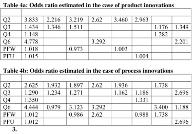
[image:27.595.84.467.490.752.2]

Tables 4a and 4b present the estimated odds ratios in the addition of extra variables in the logit formulation and for the cases of product and process innovations respectively. Specifically, the first column presents the variables and the second the odds ratios when running a logit formulation for each variable. That is if we run a logit for the case of turnover the odds ratio equals to 3.833 while if we run a logit only for exports then the odds ratio is 4.778. The other columns refer to the case of running logit models with more than one explanatory variable.

Table 4a: Odds ratio estimated in the case of product innovations

Q2 3.833 2.216 3.219 2.62 3.460 2.963

Q3 1.434 1.346 1.511 1.176 1.349

Q4 1.148 1.282

Q6 4.778 3.292 2.201

PFW 1.018 0.973 1.003

PFU 1.015 1.004

Table 4b: Odds ratio estimated in the case of process innovations

Q2 2.625 1.932 1.897 2.62 1.936 1.738

Q3 1.290 1.234 1.271 1.162 1.186 2.696

Q4 1.350 1.331

Q6 4.444 0.979 3.123 3.292 3.400 1.188

PFW 1.012 0.986 2.62 0.988 1.738

PFU 1.012 2.696