http://dx.doi.org/10.4236/cn.2013.54042
An Analysis and Computation of Optimum Earth
Geographical Coverage for Global Satellite
Communications
O. C. Eke Vincent1*, A. N. Nzeako2
1
Department of Computer Science, Ebonyi State University, Abakaliki, Nigeria 2
Department of Electronic Engineering, University of Nigeria, Nsukka, Nigeria Email: *veke39@yahoo.com
Received July 19, 2013; revised August 19, 2013; accepted August 26, 2013
Copyright © 2013 O. C. Eke Vincent, A. N. Nzeako. This is an open access article distributed under the Creative Commons Attribu- tion License, which permits unrestricted use, distribution, and reproduction in any medium, provided the original work is properly cited.
ABSTRACT
This paper presents simple mathematical mobility models for configuration of Global interconnectivity with LEO satel- lite systems. The aim of this paper is to investigate on the performance measures of the satellite mobility models re- garding optimum Global coverage arc length depending on the satellite locations relative to the four zones (quadrants) of the earth surface. A typical body of the satellite was positioned at a modified height of 780 Km from the earth surface and revolving round the earth in a circle of radius, 7160 Km was carefully studied and analytically parameterized ena- bling the generation of realistic instantaneous coverage arc lengths data. We compared the minimum required instanta- neous arc lengths for the three mobility models that should cover the geographical coverage areas of the earth. The im- pact of the satellite movements relative to the earth locations was that the instantaneous coverage arc lengths were ex- ponentially varying with time and continuously distributed within the four zones of the earth surface to provide con- tinuous coverage around one polar orbit plane and assuming operations can continue down to an elevation angle of zero degree. The advantage of the derived mobility models is achieving almost 100% global coverage as a result of the dy- namic behavior of the satellite playing an important role of providing instantaneous coverage arc lengths. This proce- dure also allows comparisons among different degrees of built-up zones of the earth surface as well as extra-polation to the different locations on the earth surface.
Keywords: Global Coverage; LEO Satellite; One Dimensional Model; Satellite Mobility Model; Central Angle; Instantaneous Coverage; Arc Length; Terrestrial Cellular Concept
1. Introduction
We are in the midst of a global information revolution brought about by the evolution of digital technology. Satellite communications systems are essential in estab- lishing the global information infrastructure. The rapidly evolving information infrastructures will play a critical role in realizing the “global village” concept of the world [1]. In the last century, mobile personal communications have enjoyed an overwhelming success by using terres- trial cellular concept. Current terrestrial wireless net- work-based personal communications services (PCS) provide telecommunications services within a small geo- graphical area [2]. To provide complete global coverage
to a diverse population, several mobile satellite systems (MSS), such as Iridium, Teledesic, odyssey and Interme- diate circular orbit (ICO) satellites have been commis- sioned [3]. In addition to providing global coverage, MSS can be connected to existing terrestrial-based telecom- munication systems to share traffics [2]. Also satellite systems represent new ambitious solutions in an attempt of interconnecting fixed networks (Internet and ATM) worldwide for supporting real-time communications [4].
Satellite communication services can be provided by Geostationary earth orbit (GEO), Medium earth orbit (MEO), or Low earth orbit (LEO) satellites. Because of its much short distance from the earth, lower power re- quirements and smaller mobility terminal (MT) size, LEO satellite system is a preferable choice [5].
*
The analysis of a satellite system, through simulation, comprises many issues [4]: some of these are the precise definition of the coverage area as the inter-satellite is moving, establishment of the inter-satellite links (if the system employs ISLs), the dynamic routing in the de- rived topology, the minimization of path switching, the establishment of the up-down link, the handoff condi- tions and finally the pattern analysis of the traffic origi- nating from or terminating at the earth stations. If the coverage area of a place must be continuous, a GEO orbit can be selected or a constellation of Non Geostationary satellite orbit (NGSO) satellites can be designed to pro- vide the necessary coverage overlap between successive satellites. Since a LEO satellite is not located at a geo- synchronous orbit, it is mobile with respect to a fixed point on the earth and it is orbiting the earth with a high constant speed at a relatively low altitude [6], which re- sults in a motion seen from a reference point over the earth. Most use circular orbits, since a constant altitude means that the satellite overhead can be used for network traffic throughout its orbit. In addition, successive satel- lites arranged in circular orbits showing the orbital plane can provide continuous coverage of a strip of ground beneath them, “street of coverage”. Many proposed sys- tems use street of coverage.
It has been observed that for a system designer to de- velop a LEO constellation which provides continuous global coverage, the following design considerations are required [6]: the length of coverage arc on the surface of the earth within the instantaneous coverage, the gain of the satellite antenna (if one beam is to illuminate this coverage), the number of satellites needed to complete a global system. However, the first requirement needed further investigation as the following constraints have also been identified [6]: orbital height of 750 Km due to user terminal power, operating time between battery charges, and satellite launcher capabilities.
It is also very important to state that several mobility models have been proposed in the recent literatures which aim to describe the movements of the satellite foot prints on the earth’s surface. In almost all the studies, one dimensional model was employed [7]. This is predicated upon the view that the rotation of the earth is negligibly compared to the satellites movement. This is a simple model to work with; however, it is only valid for services that have a short mean duration. In [8], the two dimen- sional mobility models have been proposed and em- ployed [9] which took account of the earth’s rotation. It has also been observed that the satellite to which a call will be handed over is not always the following one in the orbital plane. However, if a user is located in the over-lapping area, then it is likely due to the earth’s ro- tation that he/she will be handed over to a satellite of the contiguous orbital plane.
In our study, we intend to exploit the concept of the one-dimensional mobility models in understanding the performance of the satellite mobility models with a view of determining the optimum global coverage for mobile communications services. Thus the idea of this paper is structured to present the conceptual one-dimensional sat- ellite mobility models, and analytically in order to under- stand the performance in terms of instantaneous arc length, time and coverage parameters.
2. Theoretical Procedure
We first of all consider the conceptual satellite mobility models in conjunction with analytical and numerical so- lutions that will enable us to use satellite mobility model parameters to analyze the modifications needed for the reduction of the orbital period between any two satellites placed exactly over the reference earth point; and suffi- cient for the consideration of any possible combination of the traffic distributions and constellation patterns [6]. 2.1. Description of the Conceptual Satellite
Mobility Models
In this section, we consider the geometrical aspects of determining coverage requirements. In Figure 1 below, A spacecraft orbits at a distance, rs from the centre of the
earth C. rs is the vector from the centre of the earth to the
satellite. re is the vector from the centre of the earth to the
earth station; and d is the vector from the earth station to the satellite. These three vectors lie in the same plane and form a triangle. The central angle θ measured between rs
and re is the angle between the earth station and the satel-
lite and ψ is the angle measured from re to d. The angle α
gives the angular distance between two neighboring sat- ellites of the same orbit.
We assume that the spacecraft is a communication sat- ellite and that it needs to be in contact with an earth sta- tion located at E. In this scheme, user mobility and earth rotation speeds are ignored based on the assumption of short call holding times of circuit switched voice traffic. However, multimedia traffic has longer connection hold- ing times [1]. The surface of the earth is divided up into a grid like structure of orthogonal lines: latitude and longi- tude which describes the locations of the earth stations that must communicate with the satellites, while the co- ordinates to which an earth station antenna must be pointed to communicate with the satellite are called look angles expressed as azimuth Az and elevation El (or
) angles. The earth station antenna designers use the local horizontal plane and geographical compass points to define the azimuth angle thus giving the two look an- gles
A Ez, l
for the earth station antenna towards theE C Z
Local horizontal S
d
ψ
θ
rs
re
Figure 1. Geometry for calculating coverage area.
Using the sine rule to triangle SEC, we have that
sin 90 sin
s
r d
(1)
Which yields
cos rssin d (2) All the three parameters, , , and in “Equation (1)” above have key inputs to the architecture of the sat- ellite system [7]: The angle
d
will yield the coverage area on the surface of the earth assuming the satellite has symmetrical coverage about nadir; the distance, d will determine the free space path loss along the propagation path and will be a factor in the link budget design. The elevation angle will influence the G/T (Gain/system temperature) ratio of the antenna, the blockage probabil- ity and terrain and buildings near the antenna and the likely propagation impairments that will be encountered along the path to the satellite.
Most commercial satellite systems require that the earth stations operate above certain minimum elevation angles [6]. For example, INTELSAT G band 6/4 GHz satellites operate above 50˚. At Ku band (14/11 GHz, 14/12 GHz) INTELSAT satellites operate above a minimum elevation angle of 100˚; while the Teledesic systems operate above 40˚. Given a minimum elevation angle, and an orbital height, h
rs re
, we can setup the geometry of Figure 1 above to develop a coverage area, assuming that the satellite has a symmetrical beam aimed at nadir. The central angle , which will allow us to find the length of half of the arc under the coverage arc EZ can be found thus [6] using sine rule in Figure 1, we have:
sin re sin SEC
But angle SEC 90
1
sin sin 90 e
s
r r
Arc EZ re in radians Km (4) The diameter of the instantaneous Coverage region is given by
2Arc EZ2 re (5) And the coverage angle measured at the centre of the earth is given
2
(6)
2.2. Theoretical Analysis of the Satellite Mobility Models
[image:3.595.74.269.82.293.2]In the analysis of the motion of a satellite depicted in Figure 1 above, we consider a satellite body of mass m that is at a height, h above the earth and is revolving round the earth in a circle of radius, rs. The angular dis-
placement, in radian, is given in terms of arc length it subtends on a circular radius, rs by [10] as
s
l r
Or
s
lr (7) where is circumferential distance, a satellite body on the circle of rotation has moved (or would roll without slipping) if free to do so. This is Newton’s law of circu- lar motion. The fundamental laws of physics such as Newton’s laws of motion, is given by [10] as:
2 0 0t 1 2a
t (8) These fundamental laws are usually based on empiri- cal means, that is by observation and experiment that explains variations in physical properties and state of systems [11]. These fundamental laws define mecha- nisms of change and when combined with continuity laws for energy, mass or momentum differential equa- tions result. Hence, we employ Equation (8) above to model the motion of a satellite in a circular orbit by sub- stituting Equation (8) into Equation (7).
Thus,
2
1 0 0
1 2
s s
l r r t at
At t = 0, 00 2
1 0 0
0 0
0
1 1
2 2
2 2
where,
2
s s
s s
s
l r t at r t at
l l
r t t r t t
a a v
v
r t l
a
v (9)
s
r
0 2 d d s v r t a
l (10)
The above Equation (10) relates the rate of change of the circumferential distance of a satellite body revolving the earth to the force acting on it. This is a differential (O.D.E) equation written in terms of the variables
l t,that we are interested on predicting. However, the exact solution of Equation (10) is difficult to be obtained by simple algebraic manipulation; rather we apply advanced calculus to solve it analytically.
2.3. Analytical Modeling
The analytical solution of Equation (10) above can be obtained thus: d 2 0
d s
v
l r l
t a
Rearranging, we have 2 0
d s d
v
l l r t
a
Then integrating both sides, we have
2 0d s d
v l r a
t0
2 d
1 s d
v l r t l a
0 2 log 1 t s e r v l a
2 02 1 e
t s r v a l t
(11)
Equation (11) above is cast in a general mathematical model that expresses the essential features of the physical system that we are analyzing. Note that , is the de- pendent variable; t is the independent variable, 0
l t
, ,
s
r v are the parameters, while is the driving (or forcing) function.
a
2.4. Numerical Modeling
Alternatively, we can reformate Equation (11) above using Euler’s method [11] as follows:
The time rate of change of circumferential distance can be approximated by
11
d d
i
i i
l t l t
l l
t t t t
(12)
where and are differences in circumferential distance and time respectively computed over finite in- tervals and i , are the circumferential dis- tances at an initial time and some later time respectively.
Equation (12) is then called a finite divided difference approximation of the derivative at time, .
l
t
l t l t
i1i
Thus, substituting Equation (12) into Equation (11) gives
t
1
1
2
i i s o i i i
l t l t r v
l t
t t a
1 0
i t1
2s
i i i i
r v
l t l t l t t
a
i t t 0
3 1 1
0 1 2 2 2 s
i i i i
s
i i i
r v
l t l t l t t
a
r v
l t t
a (13)
Thus, the differential equation of Equation (11) has been transformed into an equation that can be used to determine the circumferential distance algebraically at
1
i
t using the slope and the previous values of l and t
respectively. Hence, at any time along the way,
New ValueOld Value slope St ep Size (14) 2.5. Computation of the Satellite Mobility
Model Parameters
In this sub-section, we compute the satellite mobility model parameters by recalling that in [10]:
a) 780 Km 6380 Km 60 Km
7,160, 000 m
s e
r h R
71
b) 638, 000 9.8 7464.1 m s.
7,160, 000 e e g V R r
c) 7464.1 1.04 10 3s 1
7,160, 000
s
V r
d)
2 2
2
7464.1
7.78 m s 7,160, 000 s V a r
e) The Period,
2 2 7,160, 000
6027.2 sec 100.5 min 7464.1 s r T V
f) 2 2 3.14 7,160, 000
44, 964,800 m 44964.8 Km
s
l r
2.6. Modifications
combination of traffic distribution and constellation pat- tern [10]. Hence, for our system, the length of the Global coverage is l44, 964,800 m or 44964.8 Km
and the orbital period is 100.5 minutes. [image:5.595.59.290.163.426.2](13) to get Equations (15), (16) and (17), respectively. A table of values for our l l l1, ,2 3 as well as
1 l r1 s, 2 l r2 s, 3 l r3 s
values were computed
and results tabulated as shown in Table 1 below. By inserting the numerical values of the calculated
parameters in our derived equations, we have:
Also values for our l l l1, ,2 3 as well as 1 l r1 s,
2 l r2 s
, 3 l r3 s values were computed using sta-
tistical analysis of time series and results tabulated as shown in Table 2 below.
2
1 0
3 1 2
2
2
1 2
1 7,160, 000 1.04 10 7.78
2 716, 000 389
s
l r t at
m
s t t
s t t
(15)
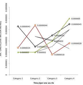
The graph of Figure 2 below shows the series of cy- clical variations of the instantaneous arc lengths of the global geographical coverage of a communications sys- tem. These series of cyclical variations occur at different points of time and are represented by quarterly time se- ries in intervals of 3 minutes as shown Table 2 below. The moving averages for Equation (9) (or Equation (15)) given by series 1 (S1), Equation (11) (or Equation (16)) given by series 1 (S2), show a rise and fall in the time interval of 0 - 3 minutes. and 3 - 6 minutes., 6 - 9 min- utes., 9 - 12 minutes, respectively while Equation (13) (or Equation (17)), shows a steadily increase in average moving from 0 - 12 minutes.
3
7
2
2
2 7,160,000 1.04 10 7464.1 7.78
1.4 10 1 e 1 e 1 e t s o t r V a t
l l t
(16)
3 1 0 1 1 3 1 7 1 2 22 7,160, 000 1.04 10 7464.1 2
7.78
2 1.4 10
i s
i i i
i
i i i
l l t
r v
l t t t
a
l t t t
l t t t
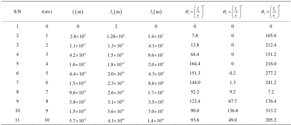
i i (17)The best simulation results were obtained using Equa- tion (13) (or Equation (17)) when compared with Equa- tion (9) (or Equation (15)) and Equation (11) (or Equa- tion (16)) respectively. The angular distance L3 ranges from 1.4 × 10⁷ to 1.4 × 10¹⁰ with moving averages from 0.000002 to 0.000005 with linear increase in length as shown in both Table 2 and Figure 2 respectively. It also has an angular coverage of 0˚ to 313˚ with 7.2˚ being optimum (as shown in Table 1).
3. Results and Discussion
This translates into having an optimum of fifty satel- lites in an orbit. A value higher than this leads to larger gaps between the footprints of different satellites, so that connection is lost during the time a ground station is Using the calculated system parameter values in Sec-
tion2.4, we therefore insert these values in our derived equations of Equation (9), Equation (11) and Equation
Table 1. A Table of values of l1
m , l2
m , l3
m vs t(sec) as well as 1, 2 3.S/N t(sec) l1 m l2 m l3 m
0 1 1 s l r 0 2 2 s l r 0 3 3 s l r
1 0 0 2 0 0 0 0
2 1 9
2.8 10 6
1.28 10 7
1.4 10 7.8 0 165.6
3 2 12
1.1 10 12
1.3 10 7
4.1 10 13.8 0 212.4
4 3 14
4.2 10 19
1.5 10 7
9.6 10 64.4 0 151.2
5 4 17
1.6 10 24
1.8 10 8
2.0 10 164.4 0 216.0
6 5 19
6.4 10 30
2.0 10 8
4.3 10 151.3 0.2 277.2
7 6 22
1.5 10 36
2.3 10 8
8.6 10 144.0 1.3 241.2
8 7 24
9.6 10 42
2.6 10 9
1.7 10 52.2 9.2 7.2
9 8 27
3.8 10 48
3.1 10 9
3.5 10 122.4 67.7 176.4
10 9 30
1.5 10 54
3.6 10 9
7.0 10 90.0 136.8 313.2
11 10 32
5.7 10 60
4.1 10 10
[image:5.595.54.539.528.736.2]Table 2. A statistical table of moving point average values for Series of instantaneous arc lengths versus time series.
Moving Point average values for Series (S1, S2, S3) of instantaneous arc lengths (L1, L2, L3) per millions: S/N Quarterly time series in intervals
of 3 mins (t(s).
Categories (CAT) of Quarterly intervals of 3 mins (t(s) in
L1 (or S1) L2 (or S2) L3 (or S3)
1 0 - 3 1 0.0000043 0.0000024 0.000002
2 3 - 6 2 0.0000025 0.0000044 0.000002
3 6 - 9 3 0.0000035 0.0000018 0.000003
4 9 - 12 4 0.0000045 0.0000023 0.000004
LEGEND: Category means a set of point values of L (L1-L3) in quarterly intervals of time. Series mean a set of cyclical variations of the instantaneous arc length point values.
0.0000043
0.0000025
0.0000035
0.0000045
0.0000024
0.0000044
0.0000018
0.0000028
0.000002 0.000002
0.000003
0.000005
0
0.
0000
01
0.
0000
02
0.
00000
3
0.
00000
4
0.
0
00005
0.
0
00006
Category 1 Category 2 Category 3 Category 4
Time,t(per one sec.tle
Series 1 Series 2 Series 3
2 per. Mov. Avg. (Series 1) 2 per. Mov. Avg. (Series 2) 2 per. Mov. Avg. (Series 3)
A
R
C
LE
N
G
TH
,L(
P
ER
M
ILLI
O
N
M
ET
R
ES
[image:6.595.149.438.257.551.2])
Figure 2. Graph of instantaneous arc length vs time.
inside such a gap. On the other hand, a low value has the effect that the period of time, in which both ground sta- tions are in the footprints of the satellites, is very short which means frequent handover between adjacent satel- lites.
To an observer on the ground, the satellite appears to have infinite orbital period. It always stays in the same place in the sky [3]. Hence the instantaneous coverage arc is exponentially increasing with time as observed in Table 1 above using Equation (13) (or Equation (17)). In [5,6], the authors found that the mean one way transmis- sion time (OTT) cannot be accurately approximated by dividing OTTs in half i.e. the variation in the OTTs are
period (0 - 10 seconds) shows that coverage angles
1, 2, 3
fall within various quadrants of the Globe.For instance, 1 covers the first and second quadrants
of the range 7.8˚ to 164.4˚, 2 covers the first and sec-
ond quadrants of the earth in the range of 0˚ - 136.8˚ while 3 covers the first, second, third and even the
fourth quadrants of the of the earth in the range of 7.2˚ - 313˚ with Equation (13) or (17). This shows the best cov- erage of the Globe.
4. Conclusions and Further Research
An in-depth analysis and computation of optimum earth geographical coverage for Global satellite communica- tions have been presented in the paper. A successful de- velopment of the satellite mobility models is presented and the performance of the satellite mobility models is evaluated in terms of the instantaneous arc length, time, and coverage angle parameters through mathematical simulations.
A comparison of the three developed satellite models has been made for developing earth geographical cover- age for satellite Global communications. We believe that an optimization technique can approximate this asym- metric variation very effectively in the instantaneous arc lengths and this is exactly an interesting point for further investigation. System performances such as global cover- age decisions, low handover rate requirements, accept- able transmission delay etc. need further research.
REFERENCES
[1] P. Chitre and F. Yegenoglu, “Next Generation Satellite Networks: Architectures and Implementations,” IEEE
Communications Magazine, Vol. 37, No. 3, 1999, pp. 30-
36.
[2] P. K. Chowdhury, M. Atiquzzama, et al., “Handover
Schemes in Space Networks: Classification and Perfor- mance Comparison,” 2nd IEEE International Conference
on Space Mission Challenges for Information Technology,
Pasadena, 17-20 July 2006, pp. 8-108.
[3] I. F. Akyildiz, H. Uzunalioglu and M. D. Bender, “Hand- over Management in Low Earth Orbit (LEO) Satellite,”
Mobile Networks and Applications, Vol. 4, No. 4, 1999,
pp. 301-310.
[4] E. Papatron, et al., “Performance Evaluation of LEO Sat- ellite Constellations with Inter-Satellite Links under Self- Similar and Passion Traffic,” John Wiley & Sons, Ltd., Hoboken, 1999.
[5] S. Karapantazis, et al., “On Call Admission Control and Handover Management in Multimedia LEO Satellite Sys- tems,” Proceedings of the 23rd AIAA International Com-
munications Satellite System Conference, Rome, 25-28
September 2005.
http//newton.ee.auth.gr/pavliodou/papers/co56.pdf [6] T. Pratt, et al., “Satellite Communications,” 2nd Edition,
John Wiley, Ltd., New York, 2003, pp. 52-432.
[7] S. Karapantazis, et al., “On Bandwidth and Inter-Satellite Handover Management in Multimedia LEO Satellite Sys- tems,” 23rd AIAA International Communications Satellite
Systems Conference (ICSSC 2005), Rome, 25-28 Sep-
tember 2005.
http//newton.ee.auth.gr/pavliodou/papers/co59.pdf [8] V. Paxson, “End-to-End Internet Packet Dynamics,”
IEEE/ACM Transactions on Networking, Vol. 7, No. 3,
1999, pp. 277-292.
[9] K. Claffy, G. C. Polyzos and H.-W. Braun, “Measure- ment Considerations for Assessing Unidirectional Laten- cies,” Vol. 4, No. 3, 1993, pp. 121-132.
[10] F. W. Sears, M. W. Zemasnsky and H. D. Young, “Uni- versity Physics,” 6th Edition, Addison Wesley, New York, 1981, pp. 181-182.