Competitiveness and the real exchange rate: the standpoint of countries in the CEMAC zone

Munich Personal RePEc Archive

Competitiveness and the real exchange

rate: the standpoint of countries in the

CEMAC zone

Lendjoungou, Francis

2 September 2009

Online at

https://mpra.ub.uni-muenchen.de/17053/

COMPETITIVENESS AND THE REAL EXCHANGE RATE: THE STANDPOINT OF

COUNTRIES IN THE CEMAC ZONE 1.

Francis LENDJOUNGOU2

(02/09/09 Version)

Abstract

This paper focuses on real exchange rate in the case of CEMAC countries. To analyze the situation in Cameroon, Central African Republic, Congo, Gabon and Chad we used annual data from 1979 to 2008. Two approaches were used related to equilibrium real exchange rate model based on fundamentals and calculations show that terms of trade, public expenditure, the degree of openness of the economy and productivity are the most important variables which influence the equilibrium of real exchange rate. Based on the estimated paths, there was a clear pattern of overvaluation before 1994, suggesting that the exchange rate adjustment was needed. Despite a relative appreciation trend during last years, the real exchange rate of CEMAC countries has not experienced an important overvaluation.

JEL Classification Numbers: C22, C53, F31, F41, O55.

Keywords: Equilibrium real exchange rate, CEMAC, FEER.

Résumé

Cette étude s’intéresse à la dynamique du taux de change effectif réel dans les pays de la CEMAC. Les analyses pour le Cameroun, la République Centrafricaine, le Congo, le Gabon et le Tchad s’appuient sur des données annuelles couvrant la période récente (1979-2008). Deux approches sont utilisées pour illustrer le modèle d’équilibre fondé sur les fondamentaux et les calculs permettent de montrer que les termes de l’échange, les dépenses publiques, le degré d’ouverture et la productivité sont les variables fondamentales influençant l’équilibre du taux de change réel. La décennie précédant la dévaluation a été caractérisée par de longues périodes de surévaluations de la monnaie, justifiant ainsi la dévaluation de 1994. En dépit d’une tendance à l’appréciation, le taux de change réel de la CEMAC n’est pas surévalué sur la période récente.

I – Introduction:

The recent continuous appreciation of the euro (the European common currency) against the dollar has given the impression that the CFA Franc has been overvalued in recent years, giving room to fear of an imminent devaluation. In fact, in 80’s there was widespread speculation that the CFA Franc would overvalued. The debate resulting from this expectation ended up with the devaluation of this currency on January 1994.

This debate is still on today. We have been witnessing a continuous rise in the value of the euro against the dollar since 2002. The value of the euro has increased by 78.4 % between January 2002 (0.88 dollar) and April 2007 (1.57 dollar). This has also caused a parallel increase in the real exchange rate of the CEMAC countries. These changes have awakened the idea of an overvaluation

1

The 6 countries of CEMAC zone are: Cameroon, The Central African Republic, Congo, Gabon, Equatorial Guinea, Chad.

2

Economist, Bank of Central African States, B.P. 1917 Yaoundé, Cameroon.

of the CFA Franc. These fears stem from the fact that the CFA Franc is pegged to the euro in a fixed parity since January 1999; making impossible for the nominal exchange rate to be used to correct macro-economic disequilibrium in the region3.

We cannot reasonably discuss the issue of overvaluation or undervaluation of exchange rate of currency without first of all, setting a reference value that will be used as the equilibrium value. The aim of this paper is to calculate the equilibrium real exchange rate and comment the possible distortions related to the economies of the Central African Economic and Monetary Community (CEMAC). Some of the questions this paper seeks to address are i) What are the determinants of real exchange rate in CEMAC countries? ii) What is the equilibrium real exchange rate? iii) The CFA Franc overvalued or not?

We can get answers to these questions by using a methodology based on fundamental variables (FEER) postulated by Williamson. In so doing, we use two approaches. The first approach estimates the short and long term parameters using the two-stage co-integration technique (Engle-Granger). The resulting parameters enable us to work out the equilibrium real exchange rate. The second approach enables us to estimate one variable representing internal balance and two others indicating external balance. This study confirms the idea of the progressive loss of control of the bargaining power that was a legacy of the 1994 devaluation. Despite the apparent appreciation of the exchange rate. the real rate of exchange has not been overvalued. There is a marked contrast between the period after devaluation in 1994 and the decade before (the 80’s) that was characterised by long phases of overvaluation. As such, we cannot expect another devaluation in the short run.

The rest of the paper will be divided into five sections. After attempting a descriptive analysis of the evolution of the real exchange rate (II), we will look summarily at certain theoretical aspects related to the dynamics of the real exchange rate (III). We then go on to calculate the equilibrium real exchange rate using the fundamental variables (IV) and the indicators of internal and external balance (V) and lastly the general conclusion (VI).

II – Descriptive analysis of the of real exchange rate:

Our period of study covers recent times from 1979 to 2008 4. During this period, there was a marked depreciation of the real effective exchange rate in all the countries in the study.

Graph 1: Evolution of the real exchange rate in 5 CEMAC countries (base 100=2000)

The analysis revealed that the countries had the following relative depreciation in their exchange rates: Congo (-13.1%), Cameroon (-18.5%) and Central African Republic (-28.5%). The hardest hit were Gabon (-50.5%) and Chad (-40.7%).

0 50 100 150 200 250

1979 1981 1983 1985 1987 1989 1991 1993 1995 1997 1999 2001 2003 2005 2007

TCR_Cam TCR_RCA TCR_Chad TCR_Gab TCR_Cgo

3_{1 euro = 655.957 CFA Franc.}

4

Analysis of the trend in real exchange rates in African countries in the CFA Franc zone in general, and those of the CEMAC region in particular, reveals two sub periods in recent years. The first sub period goes up to 1994, and the second from 1994 to this day. In this paper the abbreviations CAM, CAR or RCA, Chad, Gab and Cgo will henceforth be used to designate: Cameroon, the Central African Republic, Chad, Gabon and Congo respectively. During the first sub-period the evolution was more or less contrasting. In Cameroon for instance, there was a relative increase with peaks in 1987 and 1988 and then a progressive drop up till 1994. CAR attained its peak in 1986 while Chad and Gabon saw peak increases in 1993 and 1990 respectively. During the second sub period, a consistent slight appreciation of the real exchange rate was observed in all the countries under study. The break in this trend observed in 1994 shows that the 1994 devaluation helped all these countries to boost their competitiveness with an increased competitiveness margins rate of between 30 and 40 %.

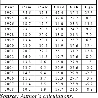
Table 1: Cumulative competitiveness margins since 19945.

Specifically, the cumulative competitive margins estimated using the real exchange rate for Cameroon, CAR, Chad, Gabon and Congo were respectively 35.6 %, 37.3 %, 47.4 %, 32.5 % and 22.3 %. These profits have been reduced progressively. In 2008, residual margins stood at 21.5 % for Gabon, 19.7 % for Chad, 10.2 % for Cameroon and 1.9 % for CAR. In the case of Congo, all the profits accruing from the devaluation were completely wiped out by 2004 (see Table 1).

Y e a r C a m C A R C h a d G a b C g o

1 9 9 4 3 5 .6 3 7 .3 4 7 .4 3 2 .5 2 2 .3 1 9 9 5 2 0 .2 1 9 .3 3 7 .6 2 2 .2 8 .3

1 9 9 6 1 8 .7 1 7 .2 3 4 .0 2 3 .3 1 3 .1

1 9 9 7 2 3 .3 2 0 .3 3 3 .8 2 4 .7 9 .9

1 9 9 8 1 8 .0 2 2 .9 3 3 .8 2 1 .3 7 .0

1 9 9 9 1 3 .4 2 8 .1 3 8 .3 2 5 .7 6 .5

2 0 0 0 2 3 .9 3 0 .5 3 4 .9 3 2 .6 1 2 .4

2 0 0 1 2 0 .7 2 7 .2 2 6 .1 3 1 .2 1 2 .8 2 0 0 2 1 6 .9 1 4 .8 1 9 .7 3 2 .6 8 .0

2 0 0 3 1 3 .8 8 . 6 1 6 .8 2 7 .9 1 .5

2 0 0 4 1 3 .7 9 . 5 2 0 .9 2 7 .6 - 2 .9

2 0 0 5 1 4 .5 9 . 4 1 6 .0 2 9 .9 - 2 .3

2 0 0 6 1 1 .3 3 . 7 1 0 .3 2 7 .7 - 3 .9

2 0 0 7 1 1 .4 3 . 5 2 0 .9 2 3 .9 - 5 .7 2 0 0 8 1 0 .2 1 . 9 1 9 .7 2 1 .5 - 8 .8

Source: Author’s calculations.

III – The equilibrium exchange rate:

III – 1: Theoretical concepts

The major difficulty in estimating the equilibrium real exchange rate is that this variable cannot be observed directly. The global strategy is thus to express this value in relation to observable and measurable variables. Thus we can distinguish several theories like the Purchasing Power Parity (PPP) 6, the natural real exchange theory (NATREX) from Stein (1994, 1995)7 or the Fundamental Equilibrium Exchange Rate (FEER). Williamson’s FEER theory (1985, 1994) remains the most used. The FEER is defined as the real exchange rate that can generate a current excess or deficit that is equal to the parallel cash flow during a given period. on condition that the internal balance of the economy is preserved and will not need protective measures against foreign exchange.

The equilibrium exchange rate is a medium term concept. In the short term situation, as a matter of fact, the exchange rate would not be equal to FEER due to the multiple factors that can affect the internal balance (the existence of a business cycle. for instance) as well as external balance (the existence of capital flow related to exchange rates differentials…). Conversely, as the effective production converges towards its potential level and capital flows tend towards their structural level, the FEER will eventually reach its equilibrium in the medium term.

5

MCt = MCt-1 – ∆TCERt, and MC1994 is the cumulative competitiveness margin in 1994 and corresponds to the variation in the real

exchange rate in 1994, where MC refers to cumulative margins.

6

The paper of Froot & Rogoff (1995) has shown that the PPA theory is invalid.

7

III-2 Brief literature review

The issue of equilibrium exchange rate in general, and the misalignment of exchange rate in developing countries. in particular, has given rise to a lot of literature especially focussing on the question of the devaluation of the CFA Franc. It is in this light that authors like Devarajan and Hinke (1994), Kiguel and Ghei (1993), Devarajan, Lewis and Robinson (1993) and Baffes et al. (1999) have expounded. The study by Tassa et al. (2002) focuses particularly on the misalignment of exchange rate noticed in 12 countries of the Franc zone. A paper by Traoré (2004) also focuses on the real equilibrium exchange rate in Burkina Faso while Gelbard and Nagayasu (2004) talks about the determinants of the exchange rate in Angola. In the case of CEMAC countries, we can cite the works of Zakar (2005) and a more recent study by Abdih and Tsangarides (2006). The latter study focuses on the estimation of the real equilibrium exchange rate in the UEMOA and CEMAC zones, and concludes that the CFA Franc is not overvalued. Linjouom (2004) proposes an interesting review in his paper on this question suggesting economic policy factors as influencing the Cameroonian situation. Finally, Bakhache et al. (2006) talks on the competitiveness in CAR.

This study takes a different view from those of all the earlier studies for two reasons: The first is that it takes into consideration each CEMAC country. The second is that it tries to estimate their real equilibrium exchange rate. This is justified by the evident link it has to the context of the recent increase in value of the euro. The countries treated in the study are Cameroon, Chad, Congo, CAR and Gabon. There is no data available for Equatorial Guinea for the period under review.

III – 3 Fundamental variables in the FEER model

This approach warrants that certain fundamental variables be put in focus. We are going to talk about the following8:

- The terms of trade (tot), defined as the ratio of export price index to import price index. In theory. the influence of the terms of trade on the real exchange rate remains very ambiguous as revealed by Baffes et al (1999). In fact, a positive change in the terms of trade (increase in export price against imports) causes an increase in supply of export goods, thus improving everything being equal, the current account which in turn causes a real exchange rate appreciation. On the other hand, an improvement in the terms of trade is seen in the increase in imports giving rise through the phenomenon of substitution (of local goods for imported ones) caused by demand. This increase can be higher than the exports, thus causing a regression of the current account and subsequently depreciation in the real exchange rate. In theory, the impact of these factors on the real exchange rate remains ambiguous and depends on the price elasticity of the demand.

- Public consumption of non tradable goods (gg). An increase in this consumption against tradable goods would have a positive impact on the real exchange rate. The increase in consumption of non tradable goods would increase the price of such goods. This will result in the increase in the rate of exchange. But some countries can expect a negative impact. In fact, in countries where imports are very high, an increase in public spending (or in consumption) can lead to an increase in the demand for tradable goods and thus a decrease in the current account and finally a depreciation of real exchange rate. Like Mongardini (1999), we used as proxy for this variable. public consumption as a percentage of the GDP. We thus have to be careful when interpreting the results connected with this variable.

- The degree of openness of the economy (open) is the sum of exports and imports as a percentage of GDP. This variable gives an insight into the country’s commercial policies (implicit and explicit trade barriers). Reduction of customs duties increases demand for foreign goods and this helps to worsen the trade deficit. If the tradable goods are perfect substitutes to the non-exchangeable ones in consumption, the real exchange rate will have to depreciate in order to re-establish external balance. This results in a negative balance.

- Investment expenditure (cf) is known to encourage economic productivity. Thus, everything being equal, an increase in investment expenditure induces the reduction in the price of tradable goods (in the medium and long term). The relationship between investment expenditure and real exchange rate ultimately depends on a much higher influence of investment expenditure on the increase in productivity of either exchangeable or non tradable goods.

- Net foreign assets (nfa): This variable depends on the capacity of the Central Bank to defend its currency. An increase in net foreign assets will cause an increase in the real exchange rate, while a decrease in net foreign assets will tend to induce a decrease in the real exchange rate. Taking into account the actual context of the CFA Franc zone can undermine the direct impact of this variable.

- Per capita rate of growth rate relative to that of commercial partners (prod) can be considered as an indicator of productivity9. This is expected to take into account the possibility of the Balassa-Samuelson effect. Improving productivity of the tradable goods sector should have a positive impact on the terms of trade. Improving productivity should lead to an increase in the real exchange rate. The end point is thus positive.

These fundamental criteria define the real equilibrium exchange rate and this relationship can be expressed by the formula:

(

)

jt i

it FONDT u

TCRE =β₀ +β₁ + (3.1)

where TCRE is Equilibrium Exchange Rate and FONDT is fundamental economic variables. Similarly. i and j designate the country and the fundamental variable respectively. Statistical analyses of the stationarity tests (ADF and KPSS) confirm the hypothesis of a unit root in nearly all the variables under study 10. We adopted the Engle & Granger two-steps method for this analysis. Alternative methods like the Johanssen (1988. 1991) and the Johanssen & Juselius (1990) methods do not appear relevant as they use autoregressive vector processes which require a longer time frame than what we have available (30 observations). On the other hand. this two-steps approach is common in similar situations11.

IV – Empirical Analysis

IV-1 Analysis of long term relation

As mentioned above. the sign of terms of trade is ambiguous. In the case in hand, there is a positive correlation between the terms of trade and the real exchange rate. This suggests that direct effects (or revenue effects) override potential substitution effects induced by the impact of terms of trade.

9_{We take into consideration 6 major partners for each of the countries in the study.}

10

The stationarity tests results can be provided by the author upon request.

11

Public consumption is positively correlated to real exchange rate. These results surely confirm the fact that government spending is usually directed towards non tradable goods sectors rather than tradable goods sectors. Invariably, the effect is a decrease in resources for the tradable goods sectors. Invariably. the effect is a decrease in resources for the tradable goods sectors.

This results in an increase in the real exchange rate. When the real exchange rate is statistically significant, the investment coefficient carries a negative sign. This is in conformity with the theory that investment contains a

huge import component. As such, an

increase in investment tends to induce an increase in the consumption of tradable goods and thus real exchange rate depreciation. The coefficient of productivity is rated positive except in the case of CAR. This positivity tends to respect the precepts of the Balassa-Samuelson effect in the countries of the sub-saharan region.

Table 2: Long term relations.

Dependent variable: Real exchange rate

Period of estimation: 1979-2008 (*)

CAR Cam Cgo Gab Chad

Constant 3.27 4.99 5.17 3.25 2.43 [0.29] 0.52] [0.45] [1.28] [0.86]

tot 0.21 -0.13 0.29 0.51

[0.04] [0.06] [0.14] [0.16]

gg 0.36 0.28 0.15

[0.09] [0.13] [0.08]

cf -0.12

[0.03]

open 0.25 -0.37 -0.22 -0.70

[0.09] [0.06] [0.08] [0.31]

nfa -0.03 -0.00 -0.00 -0.02

[0.00] [0.00] [0.01]

prod -0.20 0.44 0.33 0.43

[0.16] [0.03] [0.06] [0.20] dum94 -0.20 -0.23 -0.19 -0.16 -0.33

[0.08] [0.05] [0.07] [0.15] [0.15] R2_bar 0.91 0.92 0.73 0.82 0.66 Number of observed cases: 30. (*) The figures in braces are standard deviations.

[0.00]

The Open variable. when used as an indicator of the trade policy. enables us to consider certain factors such as the policy of quotas or exchange control. The sign in this case is largely negative suggesting that economic exposure has the tendency to reduce prices and thus cause a deterioration of the real exchange rate. But in the case of CAR, the sign is negative. This situation is probably a result of the country’s dependence on imports, which justifies the abovementioned strong import component.

The coefficients relating to net foreign assets (nfa) are nil most of the cases.

Analysis of these estimates can be done when we look at the quantified impact of the trend of fundamental variables on the interest variable. Precisely, a 1 % increase:

i) in the terms of trade, can be related to an increase in the real exchange rate

estimated at between 0.21 % and 0.51 %;

ii) in public consumption, may lead to an increase of between 0.15 % and 0.36 % in

real exchange rate;

iii) in investment, will lead to a decrease in the real exchange rate in the case of Chad;

iv) in productivity, will correspond to an increase of between 0.33 % and 0.44 % in

the real exchange rate;

v) in the degree of openness, can be related to a decrease in the real exchange rate globally estimated at between 0.22 % and 0.7 %.

IV – 2 Analysis of short term relations

We need to have an idea of the mechanisms for a return to long term forecasts. as soon as the concept is defined. From Table 3, we notice that the estimated speed of adjustment parameters are rated at 0.23 (Congo) and 0.64 (Cameroon). These values help in estimating the time (T) required for the exchange rate to reach its equilibrium point, if in the long term, this value were to deviate from its estimated curve as defined using the co-integration techniques.

Table 3: Estimates of short term relations

Dependent variable: real exchange rate (in differences)

he time T in years, is calculated using the formula: T ) adjustment of speed 1 ln( ) 1 ln( − − = α T

CAR Cam Cgo Gab Chad

ecm (-1) -0.39 -0.64 -0.23 -0.44 -0.43

[0.17] [0.19] [0.15] [0.20] [0.16]

dtot -0.12 -0.07 0.22

[0.08] [0.04] [0.16]

dgg 0.48 -0.06 0.29

[0.17] [0.04] [0.09]

dcf -0.19

[0.08]

dopen -0.29

[0.13]

dnfa -0.02 -0.01

[0.004] [0.007]

dprod 0.16

[0.15]

ddum94 -0.21 -0.27 -0.21 -0.31

[0.05] [0.02] [0.31] [0.08]

R2_bar 0.73 0.83 0.63 0.31 0.53

Number of obs.: 29. The figures in brackets are standard deviations.

Table 4: Time for returning to long term equilibrium Speed of

adjustment

T (in years) Cam 0.64 2.9 CAR 0.39 6.1 Cgo 0.23 11.5 Gab 0.44 5.2 Chad 0.43 5.3

.

Where αis the rate of dissipation of the impact of a shock (we can choose α= 95%). Thus

Camero ir

Analysis of the misalignment issue is based on the long term estimation (see table 2). By drawin

on requ es only 3 years to attain equilibrium while Congo requires 11 years to attain this equilibrium. The results for Cameroon concord with general expectations since Cameroon’s economy is the most diversified in the sub-region. For this reason, the Cameroon economy can brave the impact of a shock (internal or external). Apart from Congo, the other three economies (Gabon, CAR, and Chad) require an average of 5 years to attain this equilibrium.

V-3 The issue of misalignment I

g from Edwards’ (1994) methodology, the fundamental variables are derived from moving average method using annual data. The variables thus obtained enable us to extrapolate on the real equilibrium exchange rate12. The results are presented hereunder in graphic form (Graphs 2-4). In all of these graphs. EQS refers to the equilibrium point attained, calculated from the fundamental variables, using simple 5-year moving average. EQC represents the equilibrium obtained using the 5-year moving average, and TCR obs refers to the observed real exchange rate. Consequently, considering the initial sample, the EQS curve will cover the period from 1983-2008 while EQS covers the period from 1981 to 2006.

Graphs 2 : Observed real and equilibrium exchange rates in Cameroon and RCA (1983-2008).

C a m e r o o n

8 0 9 0 1 0 0 1 1 0 1 2 0 1 3 0 1 4 0 1 5 0 1 6 0 1 7 0 1 8 0

1983 1986 1989 1992 1995 1998 2001 2004 2007

E Q S E Q C T C R o b s

RCA 80 100 120 140 160 180 200

1983 1987 1991 1995 1999 2003 2007

EQS EQC TCR obs

Graphs 3 : Observed real and equilibrium exchange rates in Congo and Gabon (1983-2008).

Congo 80 90 100 110 120 130 140

1983 1986 198 9

199 2

199 5

1998 2001 200 4 200 7 EQS EQC TCR obs Gabon 50 70 90 110 130 150 170 190 210 230

1983 1986 1989 1992 1995 1998 2001 2004 2007

EQS EQC TCR obs

Graph 4 : Observed real and equilibrium exchange rates in Chad (1983-2008).

Chad 70 90 110 130 150 170 190 210 198 3

1986 198 9

1992 199 5

1998 200 1

2004 200 7

EQS EQC TCR obs

These graphs enabled us to draw the following major conclusions per country:

remained undervalued until 2006. There has been an apparent trend of increasing exchange rate since 2007.

CAR: We noticed intermitt

ii) ent appreciation and depreciation of the exchange rate

until the period of net appreciation between 1989 and 1993 preceding the

iii) been undervalued since 1991.

We can note a strong tendency for appreciation since 2003.

iv) evaluation helped to

maintain undervaluation up to 2004-2005. Since 2006 the currency has shown a

v) of the real exchange rate between 1988

and 1993. Since the devaluation, the real exchange rate has appreciated without

In the fina xchange rate in all the countries was not

overvalued. But data obtained for the recent years shows a tendency towards the appreciation of the exchan

al and external balance: An alternative balance evaluation method.

es carried out by the IMF in the 1970s, Williamson defined the concept of the fundamental equilibrium exchange rate as the real exchange that enables an economy to simulta

it. The reader can refer to works by authors

tical methods are much criticised for their lack of economic bases and their sample queue properties, while identification methods are challenged for the volatility of their resultant equilib

of the current balance. But this definition can only be pertinent if we consider very long term equilibrium (14). A

devaluation of the CFA Franc. There has been a perceptible trend towards appreciation since 2002 and this seems to be linked to the increased price of imports following the rise in the value of the euro.

Congo: At the time of devaluation. the currency had

Gabon: The graphs show an overvaluation in 1992-1993. D

slight appreciation of real exchange rate.

Chad: We noticed a marked overvaluation

going beyond the equilibrium value. It is worth noting that this economy registered a 9 % price decrease in 2007.

l analysis, it was observed that the real e

ge rate.

V – The intern

V-1 Overview

Following studi

neously attain internal and external balance in the medium term. The major difficulty resides in the determination of the said internal and external balance: the level of potential economic growth and the level of sustainability of the current account.

Let’s take a look on the different ways of calculating the potential GDP. The resultant potential GDP will depend on the method used to calculate

like Bouthevillain (1995) or Baghli et al (2002) for an overview on methodologies. However, the most commonly used are those that obey statistical principles based on the use of i) purely statistical techniques using Hodrick and Prescot (HP) or Beveridge and Nelson filters; ii) structural VAR based on identification methodologies like that of Blanchard and Quah (1989); iii) structural approach using the production function based on growth factors and efficiency of production.

Statis

rium variables. It therefore becomes difficult to develop a third approach for developing countries due to lack of data. On our part, we used the HP filter to estimate potential GDP13.

The level of sustainability of the current account is usually linked to the equilibrium

deficit of the current account is not a bad idea in itself. Disequilibrium in current account is

13

The smooth parameter considered is equal to 100.

14

not a real indicator of a trade crisis. Milesi-Ferreti andRazin (1996) define the non-sustainability of current account deficit if maintaining it makes the country insolvent. and thus the expected value of the market surplus is lower than the actual value of the external debt. This has caused Cartapanis. Dropsy and Mametz (1999) to define the target cc* of current account as:

g Dext g cc + × − = 1 *

where g and refer to the economic growth rate and the external debt respectively. On our pa

Dext

rt. we consider a slightly different approach used by Borrowski, Couharde and Thibault (1997). The level of the debt ratio to be stabilised d* is defined in relation to the growth rate in the economy and the current deficit. The debt ratio (D) against the GDP (Y) is given as: d=D/Y or as a

function of the growth rate

Y Y D d D d ∆ = ∆ = ∆

. The debt stabilisation ratio implies that ∆ =0 d

d .

Considering that the variation of debt is equal to the current deficit (CA), we can thus write:

g Y CA Y CA 1 −

available. To partially overcome this difficulty we consider in this paper (as a variant), a 5-year moving average.

Y Y

d* = ×

∆

= . Since most CEMAC countries are oil producers, the concept of

sustainability or external balance naturally refers to the non-oil economy. But this variable is hardly

-2 Estimating the equilibrium exchange rate:

Taking into consideration a variable that reflects external balance and another that brings out interna

V

l balance will enable us to approach the path to the equilibrium exchange rate. In this way we can use the following equation for each country:

t t t

t PIBHP d u

TCRE =β₁ +β₂ *+ (5.1)

Where TCRE is the equilibrium rate of exchange. PIBHP is the potential production calcula

able 5: Estimating the equilibrium exchange rate

Subsequently, d* is replaced by the 5-year moving average of current account as a percentage of GDP and has been denoted as MA.

Cameroon CAR Chad Gabon Congo

ted using the Hodrick Prescot filter method and d* is the external balance variable defined above. In table 5. there is a constant that is not presented which has been taken into consideration. The sign of potential production variable is not the one expected. However. when the constant is omitted. all the variables have the expected sign except the variable d* for Gabon (Appendix 2).

T

Dependent variable: ln(TCR) (*) Period: 1981- 2008

GDP -0.23 -1.545 -0.363 -1.551 -0.295

[0.182] [0.384] [0.099] [0.135] [0.114]

d* -0.098 -0.027 -0.016 -0.01 -0.003

[0.033] [0.031] [0.021] [0.025] [0.003]

Rbar2 0.29 0.42 0.34 0.84 0.16

able 6: Estimating the equilibrium exchange rate

ependent variable: ln(TCR) (*) eriod: 1981- 2008 (15)

es, the GDP variable itted. all the other variables now lts can be seen in the table in ppendix 2.When we base our calculations without the constant on regressions, we take up analysis

thod, this successive overvaluation goes back to 1981. This unidirectional misalignments (cumulating to between 107

ii)

justify the devaluation in 1994. But by 1994, we cannot clearly distinguish any period during which the real exchange rate observed was

iii)

aluation. However, there is progressive appreciation of the real exchange rate.

iv)

v) shows a period of net overvaluation until

undervaluation (from 2007-2008).

T

D P

Table 6 integrates a constant which is not represented here. For all the countri does not have the expected sign. However, when this constant is om

have the expected sign, except the d* variable for Chad. The resu A

of misalignment. This analysis enables us to understand why we should not expect devaluation in the short term. This analysis is introduced using graphs got from Appendices 3 to 7. Major lessons drawn from these analyses by country can be summarised as:

i) Cameroon: Analysis of the graph (appendix 3) for Cameroon reveals that the 8

years preceding the devaluation saw consecutive overvaluation of the real exchange rate. According to the second me

and 110 % between 1986 and 1993) justified the devaluation of 1994. During the period after 1994. the longest period of overvaluation lasted only 4 years (1996-1999) followed by 7 years (2000-2006) of undervaluation. However, pressure was noticeable at the end of this period. But it cannot be compared with the trend before the devaluation.

CAR: The graph (appendix 4) shows that the last 13 years were characterized by virtually consecutive overvaluation cumulating to a total of between 123 % and 201 %. These amounts

higher than the real equilibrium exchange rate. However, we also notice a trend of appreciation of the real exchange rate.

Congo: The graph (appendix 5) clearly defines two sub-periods. The first extending up to 1993 characterised by overvaluation, and the second stretching from 1994 to 2008 showing underv

Gabon: The real exchange rate shows an overvaluation until 1994, and then undervaluation until the end of the period.

Chad: The graph (appendix 7) clearly

1993. During the period starting from 1994, there is overvaluation for 5 years between 2002 and 2006 followed by severe

C a m e r o o n C A R C h a d G a b o n C o n g o

- 1 .5 1 - 0 .6 4 1

[0 .1 6 7 ] [0 .1 1 9 ]

.0 8 6 - 0 .0 4 6 0 .0 0 5 - 0 .0 0 1 0 .0 1 2

[0 .0 2 0 ] [0 .0 3 6 ] [0 .0 0 6 ] [0 .0 0 4 ] [0 .0 0 3 ]

R b a r 2 0 .4 9 0 .4 4 0 .3 4 0 .8 3 0 .5 0

( * ) G D P a n d M A r e p r e s e n t th e p o te n tia l p r o d u c tio n a n d th e e x te r n a l b a la n c e v a r ia b le s r e s p e c t iv e ly . T h e fig u r e s in b r a c k e ts r e p r e s e n t th e s t a n d a r d d e v ia tio n s .

G D P - 0 .0 1 1 - 1 .3 3 4 - 0 .2 8 8

[0 .4 3 4 ] [0 .1 6 0 ]

[0 .1 6 5 ]

M A - 0

15

In summary, this approach enables us to justify the devaluation of 1994. In fact, in all the tudy, we observe a net overvaluation of the real exchange rate during the decade The duration of consecutive annual overvaluations and the associated cumula countries under s

preceding 1994. tive

degrees were some of the factors that justified the devaluation of 1994. This assertion has always been a

he debate on the equilibrium exchange rate for countries of the franc zone has become a very important subject of interest in the actual global context dominated by the increase in exchange focus on CEMAC countries, the major findings of this paper are hinged on of 3 main points:

ii) the recent period does not show a marked overvaluation as it was the in the 1980s.

iii) the elasticities of internal balance variables are of higher value than those of

These findings suggest that to be primed against an increase in real exchange rate and thus

overva n of

reforms in the v licies will enable us to have control over the cost of

factors of production and thus enable us gain in competitiveness. The process of diversification of produc

topic of debate in different studies carried out on the real exchange rate of countries in the CFA Franc zone. During the recent period, the duration of the phases during which there was overvaluation of the real exchange rate are very short. Consequently, analysis show a different trend from the one observed between the decade preceding the 1994 devaluation and recent times. Generally, the real exchange rate has not been overvalued in recent times. These two arguments prove that devaluation is not warranted again. However, there has been a gradual trend towards a slight exchange rate appreciation over the last years.

VI – CONCLUSION

T

value of the euro. With

i) there is a loss of competitiveness that is reflected in the almost continuous increase in the real exchange rate;

Thus, we cannot expect a new devaluation in the short run;

external balance variables.

luatio CFA Franc, we need to work hard to improve on structural and institutional

arious economies. These po

References

[1]- Abdih Y. and C. Tsangarides. 2006, « FEER for the CFA Franc ». IMF Working Paper

No.06/236. (Washington: International Monetary Fund).

[2]- Ba awi I. and O’Connell S.(1997) : « Single-equation estimation of the equilibrium

se and Le Bihan H. (2002) : « PIB

re aux outputs gaps et aux cibles de balance courante : Méthodologie et estimation pour les

ocks,

0. ffes J., Elbad

real exchange rate ». Working paper. 08/20/97. World Bank.

[3]- Bakhache S., Kalonji K., Lewis M. and Nachega J.C. (2006), « Assessing competitiveness

after conflict: The case of the Central African Republic », IMF Working paper WP/06/303.

December, International Monetary Fund.

[4]- Baghli M., Bouthevillain C., De Brandt O., H. Frais

potentiel et écart de PIB : Quelques évaluations pour la France », NER Banque de France N° 89.

[5]- Banque Mondiale (1984): Programme d’action concertée pour un développement stable de

l’Afrique au sud du Sahara , Washington D.C.

[6]- Bouthevillain C. (1995) : « Une datation des cycles de croissance des grands pays

industrialisés ». Document de travail N° 95-2. Direction de la Prévision, Ministère de l’Economie, France.

[7]- Blanchard O. and D. Quah (1989) : « The dynamic effects of aggregate demand and supply disturbances », American Economic Review, vol. 79. 655-673.

[8]- Borowski D., C. Couharde and F. Thibault (1997) : « Sensibilités des taux de change d’équilib

grands pays industrialisés », Document de travail, N° 97-3, Décembre 1997, Direction de la Prévision, France.

[9]- Cartapanis A., Dropsy V. and Mametz S.(1999) : « Indicateurs d’alerte et crises de change : Analyse comparée des économies d’Europe Centrale et Orientale (1990-1997) et d’Amérique latine et d’Asie de l’Est (1971-1997) », Revue économique, vol. 50. Novembre 1999, p.1237-1254.

[10]- Clark P. and Mac Donald R. (1998): « Exchange rates and economic fundamentals : A

methodological comparaison of BEERs and FEERs », IMF Working Paper n°98/67, May,

International Monetary Fund.

[11]- Devarajan Shantayanan, Geoffery D. Lewis and Sherman Robinson (1993): « External sh

purchasing power parity and the equilibrium real exchange rate », The World Bank Economic

Review, Vol. 7. No. 1. 45-63, World Bank, Washington. DC.

[12]- Devarajan. S. and L. Hinkle (1994): « The CFA Franc Parity Change: An Opportunity to Restore Growth and Reduce Poverty », Afrika Spectrum 29 (2): 131-51.

[13]- Edwards Sebastian and Savastano Miguel (1999): « Exchange rates in Emerging economies : what do we know ? what do we need to know? », NBER Working paper 7228, Princeton University Press.

[14]- Edwards S. (1989) : Real exchange rates. devaluation and adjustment : exchange rate policy in developing countries , Cambridge, Mass. MIT PRESS.

[15]- Edwards S. (1994) : « Real and monetary determinants of real exchange rate behavior : Theory and evidence from developing countries », in Estimating equilibrium exchange rate, ed. By John Williamson.

[16]- Feyzioglu T. (1997): « Estimating the equilibrium real exchange rate: an application to Finland », IMF Working paper WP/97/09, (Washington: International Monetary Fund).

[17]- Froot K. and Roggoff K. (1995), « Perspectives on PPP and the long run real exchange rate ».

in Grossman G. and Rogoff K. (eds), The Handbook of International Economics, vol. N°3,

Amsterdam, North Holland Press.

[18]- Gelbard E. and Nagayasu J. (2004): « Determinants of Angola’s real exchange rate 1992-2002 », The Developing Economies, XLII-3 (September 2004) 392-404.

[19]- Johansen S. (1988): « Statistical analysis of cointegration vectors », Journal of Economic Dynamics and Control, vol.12. pp.231-254.

[21]- Johansen S. (1995): Likelihood based inference on cointegration in the vector autoregressive model, Oxford University Press.

[22]- Johansen S. (1988): « Statistical analysis of cointegration vectors », Journal of Economic Dynamics and Control, vol.12, pp.231-254.

[23]- Johansen and Juselius (1990): « Maximum likelihood estimation and inference on cointegration with applications to the demand for money », Oxford Bulletin of Economics and

) : « Devaluations in Low-Income Countries » World

hiers de recherche N° 2004-03, Eurisco, Université Paris Dauphine.

The recent float from

mple? », Journal of International Economics, 14 (1-2), p.3-23.

).

Burkina », Document de Travail, Banque des Etats de

sassa C., Yamb B. and Kouezo B. (2002): « The misalignments of real exchange rates in the

The exchange rate system », Policy analysis in international

CFA zones », World Bank Policy Research Working paper N°3751.

Statistics, vol.52. pp. 169-210.

[24]- Kiguel. Miguel and Nita Ghei (1993

Bank Policy Research Working Paper 1224, World Bank, Washington. DC.

[25]- Linjouom M. (2004) : « Estimation du taux de change réel d’équilibre et choix d’un régime de change pour le Cameroun », Ca

France.

[26]- Lothian J. and Taylor M. (1996): « Real Exchange rate behavior:

perspective of the past two centuries », Journal of Political Economy 104(3), p.488-509.

[27]- Meese R. et Rogoff K. (1983) : « Empirical exchange rate models in the seventies : Do they fit out of sa

[28]- Milesi-Ferreti G.M. et Razin A. (1996) : « Current account sustainability : Selected East Asian and Latin American experiences », IMF Working paper, WP/96/110.

[29]- Mongardini J.(1998) : « Estimating Egypt’s equilibrium real exchange rate », IMF Working paper. WP/98/5, (Washington: International Monetary Fund).

[30]- Paiva C. (2001): « Competitiveness and the equilibrium exchange rate in Costa Rica », IMF Working paper, WP/01/23, (Washington: International Monetary Fund

[31]- Stein J. (1994): « The natural real exchange rate of the dollar and determinants of capital flows », in Williamson J. (1994. op. Cit).

[32]- Stein J. and Allen P. (1995), Fundamental determinants of exchange rates, Oxford University Press.

[33]- Traoré Antoine (2004) : « Calcul du taux de change effectif réel et estimation de son niveau d’équilibre : une application au cas du

l’Afrique de l’Ouest (BCEAO). [34]- T

franc zone countries : An empirical analysis », African Economic Consortium AERC/CREA. Biannual Research Workshop, Nairobi, Kenya.

[35]- Williamson J. (1985): «

economics N°5, June, Institute for International Economics, Washington.

[36]- Williamson J. (1994): Estimating equilibrium exchange rates. Institute for International Economics. Washington.

[37]- Willet T. (1986): « Exchange rate volatility. international trade and resource allocation », Journal of International Money and Finance, (supplement). 5 (mars).

[38]- Zafar A. (2005) « The impact of the strong euro on the real effective exchange rates of the two francophone african

ANNEX 1: Estimation of table 5 without constant.

Cam Rca Chad Gab Cgo

PIB 0.169 0.185 0.179 0.176 0.178

[ 0 [

*

[0.034] [0.038] [0.029] [0.064] [0.004] 0.001] [ .001] [0.002] 0.002] [0.001]

d -0.115 -0.074 -0.042 0.059 -0.002

ANNEX 2: Estimation of table 6 without constant.

Cam Rca Chad Gab Cgo

PIB 0.158 0.167 0.184 0.180 0.177

[0.002] [ .005] [0.002] 0.002] [0.002] 0 [

CA* -0.094 -0.118 0.02 -0.028 -0.001

[0.016] [0.034] [0.004] [0.007] [0.003]

ANNEX 3: Graph of equilibrium real exchange rate in Cameroon (1981-2008) (16).

4 .5

4 .6 4 .7 4 .8 4 .9 5 .0 5 .1 5 .2

1 9 8 5 1 9 9 0 1 9 9 5 2 0 0 0 2 0 0 5

L T C R C A M C A M _ M A 2 C A M _ D S T A R 2

16

ANNEX 4: Graph of equilibrium real exchange rate in CAR (1981-2008).

4 .5 4 .6 4 .7 4 .8 4 .9 5 .0 5 .1 5 .2 5 .3

19 85 19 90 19 95 2 00 0 2 00 5

LTCRRCA RCA _ M A 2 RCA _DS TA R 2

ANNEX 5: Graph of equilibrium real exchange rate in Congo (1981-2008).

4 .5 4 .6 4 .7 4 .8 4 .9 5 .0

1 9 8 5 1 9 9 0 1 9 9 5 2 0 0 0 2 0 0 5

ANNEX 6: Graph of equilibrium real exchange rate in Gabon (1981-2008).

4.5 4.6 4.7 4.8 4.9 5.0 5.1 5.2 5.3 5.4

1985 1990 1995 2000 2005

LTCRG AB G AB_MA2 G AB_DSTAR2

ANNEX 7: Graph of equilibrium real exchange rate in Chad (1981-2008).

4.4 4.5 4.6 4.7 4.8 4.9 5.0 5.1 5.2 5.3

1985 1990 1995 2000 2005

ANNEX 8: Estimation of misalignment rate (in percent) from annex 2 and 3 (*).

Cameroon Rca Congo Gabon Chad

MA d* MA d* MA d* MA d* MA d* 1981 -2.7 11.8 35.4 27.5 20.8 21.3 52.1 43.7 26.0 37.5 1982 -10.7 8.7 28.9 26.8 18.7 19.2 53.3 44.3 13.1 27.4 1983 -10.3 11.8 29.7 43.5 14.1 14.7 51.3 40.6 10.0 27.3 1984 -9.3 10.8 16.6 25.1 16.9 16.8 44.2 35.2 21.9 40.7 1985 -6.8 16.6 22.4 29.0 15.7 16.8 39.3 45.2 25.6 43.0 1986 6.9 29.4 10.1 10.9 16.6 16.6 36.6 48.0 12.1 22.8 1987 15.0 15.7 2.0 17.9 16.0 16.3 22.2 48.3 9.1 17.5 1988 16.6 26.2 -1.8 21.4 15.9 15.2 -3.3 22.5 16.2 24.9 1989 7.8 15.6 -0.2 16.0 15.3 15.7 -6.9 27.6 8.2 19.6 1990 14.4 14.4 11.8 19.8 12.8 9.5 5.1 37.6 5.5 18.2 1991 13.8 12.8 12.2 3.3 1.8 5.4 -6.2 18.2 4.8 16.4 1992 22.3 15.8 11.3 6.4 2.2 4.3 -11.1 15.1 13.0 19.2

1993 13.2 -22.8 8.7 7.6 1.0 -1.2 -6.4 3.4 19.1 22.7

1994 -27.2 -26.2 -38.8 -36.2 -24.8 -23.8 -39.5 -33.8 -43.1 -39.2

1995 -1.6 -13.6 -24.1 -18.0 -12.3 -10.4 -26.5 -16.5 -31.9 -27.4 1996 2.3 -10.3 -18.0 -27.4 -17.7 -16.1 -20.3 -22.0 -26.4 -25.1 1997 3.1 -16.7 -13.8 -19.5 -14.7 -13.1 -15.1 -21.4 -24.1 -21.7 1998 11.1 -7.3 -28.3 -17.6 -11.9 -11.1 -18.7 -20.4 -24.5 -26.9 1999 10.2 3.6 -30.9 -28.4 -11.4 -10.8 -22.8 -44.9 -29.4 -40.4 2000 -6.1 -17.8 -20.8 -31.5 -17.3 -17.5 -24.5 -34.3 -24.3 -19.6 2001 -7.9 -12.4 -15.5 -27.4 -17.8 -18.5 -25.9 -43.9 -8.6 -19.5 2002 -14.3 -11.4 -1.6 -2.5 -13.6 -14.3 -29.3 -34.3 7.2 7.6 2003 -10.4 -7.3 13.1 -16.8 -7.8 -9.1 -12.5 -17.3 23.6 4.6

2004 -12.0 -4.3 11.6 -5.7 -3.7 -5.2 -11.3 -27.8 19.7 -19.8

2005 -17.2 -6.3 -1.1 -9.1 -4.9 -6.4 -14.0 -31.4 16.0 -21.3

2006 -6.5 -12.6 1.6 -7.1 -4.0 -5.5 -8.3 -25.0 11.6 -12.2

2007 3.1 -13.3 -5.4 -2.8 -3.3 -5.0 -1.6 -23.9 -14.9 -39.5

2008 3.4 -10.0 -14.1 -4.2 -0.8 -2.2 3.6 -27.4 -32.9 -29.6