Munich Personal RePEc Archive
A Quantitative Analysis of
Suburbanization and the Diffusion of the
Automobile
Kopecky, Karen A. and Suen, Richard M. H.
5 January 2009
Online at
https://mpra.ub.uni-muenchen.de/13258/
A Quantitative Analysis of Suburbanization and the Diffusion of the
Automobile
Karen A. Kopecky∗ and Richard M. H. Suen†
January 2004
Version: January 2009
Abstract
Suburbanization in the U.S. between 1910 and 1970 was concurrent with the rapid diffusion of the automobile. A circular city model is developed in order to access quantitatively the contribution of automobiles and rising incomes to suburbanization. The model incorporates a number of driving forces of suburbanization and car adoption, including falling automobile prices, rising real incomes, changing costs of traveling by car and with public transportation, and urban population growth. According to the model, 60 percent of postwar (1940-1970) suburbanization can be explained by these factors. Rising real incomes and falling automobile prices are shown to be the key drivers of suburbanization.
JEL Classification Nos: E10, 011, N12, R12
Keywords: automobile, suburbanization, population density gradients, technological progress
Subject Area: Macroeconomics
∗Department of Economics, Social Science Centre, Room 4071, The University of Western Ontario, London, Ontario,
N6A 5C2, Canada. Email: [email protected].
† Department of Economics, Sproul Hall, University of California, Riverside, CA 92521-0427. Email:
1
Introduction
Suburbanization has been observed in cities throughout the United States since the late nineteenth
century when omnibus, commuter railroads and streetcars were first implemented. But technological
progress in transportation made its biggest contributions during the twentieth century with the
inven-tion of the automobile and later the modern highway system. The adopinven-tion of the private vehicle as the
dominant form of transportation in the United States, combined with rising income levels, encouraged
movement to less dense areas where housing was more affordable. The goals of this paper are to (1)
measure the contribution of automobiles to suburbanization during the postwar (1940-1970) period, and
(2) quantify the relative contributions of falling automobile prices, rising real incomes, changing costs
of traveling by car and with public transportation, and urban population growth to suburbanization
during the 1910 to 1970 period.
To achieve these goals, a monocentric city model is constructed in which consumers with different
income levels can choose their residential location and mode of transportation. The model is calibrated
to be consistent with, among other things, changes in car-ownership rates, prewar (1910-1940)
sub-urbanization rates, and a number of statistics on commuting and travel. The calibration method is
now commonly used in quantitative macroeconomic studies. In the urban economics literature,
Chat-terjee and Carlino (2001) adopt this method to explain the changes in employment densities across
metropolitan areas in the postwar United States. The calibration method is particularly useful for the
current study due to the paucity of data for the early years. Under the baseline calibration the model
predicts that rising real wages, falling prices of automobiles, changes in the costs of traveling by car
and public transit, and population growth can account for 60 percent of postwar suburbanization. A
series of counterfactual experiments reveal that the rise in real incomes and fall in automobile prices
are the key drivers of suburbanization while the growth in urban population has very little impact.
1.1 Suburbanization
Suburbanization refers to the spreading of urban population and employment from the central cities
to satellite communities called suburbs.2 This movement results in an increased dispersion of urban
population and employment over a land area. Although employment and population tend to move
simultaneously, jobs have been more concentrated than residents throughout the period in question.
2
As late as 1950, 70 percent of jobs in metropolitan areas were located in the central cities while only
57 percent of residents were located there. In 1970, 55 percent of jobs were located in the central cities
compared to only 43 percent of residents (Mieszkowski and Mills, 1993). Thus, while the majority of
firms were still concentrated in the central cities in 1970, a large portion of the urban population had
already relocated to the suburbs. In light of these developments, the current study focuses on explaining
the suburbanization trend of the urban population and abstracts from employment decentralization.3
Measuring Suburbanization To measure the extent of suburbanization, researchers typically focus on how the population density function changes over time. The population density function is assumed
to take the negative exponential form
D(x) =ae−bx, (1.1)
where D(x) is the population density (total residential population divided by total land area) at
distancexfrom the city center. The parameteraprovides an estimate of the density at the city center.
The parameter b, known as the population density gradient, measures the rate at which population
density falls with distance.4 The extent of suburbanization that occurred over a period of time can be
captured by the percentage change in the population density gradient.
Historical Facts Suburbanization is a widely observed phenomenon in the United States, as well as many other countries around the world. In the United States, the growth of suburban areas began in
the nineteenth century. Taylor (1966) reports that, between 1830 and 1860, population growth rates
in the suburbs of New York, Philadelphia and Boston were much higher than in the central cities and
that by 1860, 38 percent of Boston’s population and 31 percent of New York’s lived in suburban areas.
Using the exponential density function described above, Mills (1972) finds that the population density
gradients of Baltimore, Milwaukee, Philadelphia and Rochester have been consistently decreasing since
1880. Decreasing population density gradients have been observed for almost all American cities during
the period 1910 to 1970, making it the most intensive period of suburbanization in the United States.
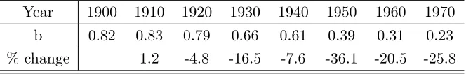
Table 1 shows the evolution of the average population density gradient of forty-one American cities
between 1900 and 1970.5 The density gradient declined by 77 percent over this period, declining most
3
Theoretical studies that allow identical firms and households to choose their locations simultaneously include, among others, Fujita and Ogawa (1982) and Lucas and Rossi-Hansberg (2002). Incorporating household heterogeneity and different modes of transportation into these models would greatly increase the complexity of the analysis and compu-tation.
4
The exponential population density function was first introduced in Clark (1951). Subsequent studies have applied it to measure suburbanization in urban areas worldwide. See Mills and Tan (1980) for a survey of these results. See Mills (1972) and McDonald (1989) for more details on the estimation method.
5
Table 1: Mean Gradients for Forty-One Cities That Were Metropolitan Districts in 1900.
Year 1900 1910 1920 1930 1940 1950 1960 1970 b 0.82 0.83 0.79 0.66 0.61 0.39 0.31 0.23 % change 1.2 -4.8 -16.5 -7.6 -36.1 -20.5 -25.8
Source: Edmonston (1975, p. 68).
rapidly during the 1940’s when it fell by 36 percent.
Part of the decline in population density gradient is due to the growth of urban population between
1900 and 1970. At the beginning of the twentieth century, only 40 percent of Americans lived in urban
areas. However, by the late 1970’s, more than 70 percent did. While the total U.S. population grew
at an average annual rate of 1.4 percent during this time period, the comparable growth rate of urban
population was 2.3 percent. As the urban population increases, cities must expand spatially in order
to accommodate more people. Population growth, however, cannot explain the entire suburbanization
trend. Edmonston (1975) finds a consistent decline in population density gradient even after controlling
for city population size. This shows that there are factors other than population growth that contribute
to the suburbanization trend.
Theories of Suburbanization Suburbanization has been studied extensively over the years by urban economists, geographers and historians. Some of the most popular theories are discussed below.
The standard theory of suburbanization, which is also the one developed and assessed in this paper,
proposes that the phenomenon is driven by a combination of technological progress and rising incomes.
Transportation innovations such as streetcars, commuter rails, subways and automobiles affect the
spatial distribution of households by lowering the time cost of intra-urban travel. In response to lower
transportation costs, those who can afford the new technology move to outlying areas where cheaper
land translates into more spacious houses and larger yards. As real incomes rise and technological
progress drives a decline in the relative price of the new transport mode, more urban households adopt
it and relocate to suburban areas. This process drives the expansion of metropolitan areas and the
decline in their population density gradients.
The rise in real incomes in the United States since the nineteenth century has been well-documented.
introduced into American cities since the 1830’s.6 Studies supporting the standard theory of
sub-urbanization during the nineteenth century include the following. Warner Jr. (1962) notes that the
introduction of streetcars into Boston likely caused the first major movement of affluent households
to the suburbs during the 1850’s and the 1860’s. While Taylor (1966) argues that the introduction of
omnibuses, commuter railways and streetcars between 1830 and 1860 encouraged city-dwellers to live
in outlying areas and travel to work.
By far the biggest technological breakthrough in transportation came with the invention of the
automobile at the dawn of the twentieth century. The extensive suburbanization observed during the
decades that followed was concurrent with the diffusion of automobiles into American households.7
Glaeser and Kahn (2004) assert that the root of urban sprawl is the “technological superiority of
the automobile.” Using cross-sectional data from the United States as well as other countries, these
authors find a strong positive correlation between low population density and automobile use. A more
recent innovation in transportation technology was the development of highway systems, which were
introduced into the United States during the 1950’s. Using data from the period 1950 to 1990,
Baum-Snow (2007a) estimates that the construction of a new highway which passes through a city’s center
reduces the center’s population by about 18 percent. As Baum-Snow states, the results of his study
suggest that the construction of interstate highways can account for about one-third of the decline in
the share of the metropolitan population living in central cities during the 1950 to 1990 period.
Along with technological progress in transportation, there is also evidence that rising real incomes
played an important role in twentieth century suburbanization. Margo (1992) estimates that 43 percent
of suburbanization in the United States between 1950 and 1980 can be explained by the increase in
household income over this period.
The accelerated rate of suburbanization that occurred during the postwar period has inspired the
development of other theories which attribute suburbanization to the social and economic factors that
are peculiar to the postwar United States. Two common forms of these theories are described below.
Between 1940 and 1970, there was a massive migration of black, southern households to the central
urban areas in the north. This happened at a time when suburbanization of white households was
at its peak. These observations inspired the so-called “white flight” theory, which states that whites
6
The first major innovation in mass transportation was the omnibus, which was commonly used in American cities during the 1830’s. The following decades witnessed the introduction of commuter railroads and streetcars. For more details on these early inventions see Taylor (1966). The next major innovation in intra-urban transportation was rapid transit. The first underground rapid transit line in the United States was opened in Boston in 1897.
7
Table 2: Percentage of Households Owning at Least One Car, 1910-1970.
Year 1910 1920 1934-36 1950 1960 1970
% 2 33 44 59 77 82
Source: See Car-Ownership in the Data Section of the Appendix.
relocated to the suburbs as a response to the inflow of black migrants.8 In a recent study, Boustan
(2007) estimates that about 20 percent of postwar suburbanization can be explained by this theory.
Other studies suggest that postwar suburbanization is largely a response to the deteriorating social and
economic conditions in the central cities (Bradford and Kelejian, 1973; Frey, 1979; Grubb, 1982; Mills
and Lubuele, 1997; Cullen and Levitt, 1999).9 According to this theory, affluent households move to
the suburbs to avoid problems in the central cities such as racial tension, high crime rates, low-quality
public schools and high taxes. While the “white flight” and “central city disamenities” theories may
explain some aspects of suburbanization, such as its accelerated rate in the early postwar period, the
importance of these theories as primary explanations of suburbanization has been called into doubt by
several authors (Mills and Price, 1984; Mieszkowski and Mills, 1993; Glaeser and Kahn, 2004). The
massive inflow of black migrants is a postwar phenomenon but the trend of suburbanization had begun
long before World War II. In addition, suburbanization is observed in places that are not plagued by
racial tension and crime. For instance, the rate of violent crimes is much higher in the United States
than in Canada but metropolitan areas in the two countries decentralized at similar rate during the
period 1950 to 1975 (Goldberg and Mercer, 1986).
1.2 The Diffusion of the Automobile
The first automobiles entered the United States market in the late 1890’s, initiating an adoption process
that would continue throughout the twentieth century. In the early 1900’s, the automobile, selling at
more than 5 times average annual household earnings, was considered more as a toy for the rich than
as a realistic mode of transportation. Even by 1910, only approximately 2 percent of American families
owned a car. Starting in the 1910’s, however, the rate of car-ownership began to increase quickly, driven
8 There is a large literature in sociology and urban geography which examines the causes and consequences of “white
flight” over the period 1950 to 1970. For instance, Frey (1979) and Marshall (1979) analyze the factors that cause white people to relocate to the suburbs. Guest (1978) documents the changing racial composition in U.S. cities between 1950 and 1970, while Sorensen, Taeuber and Hollingsworth Jr. (1975) and Farley (1977) report the extent of racial segregation during this time period.
9
Lowest Second Third Fourth Highest 0
20 40 60 80 100
P
e
r
c
e
n
t
o
f
Gr
o
u
p
Incom e Quintile
[image:8.612.193.432.58.265.2]1952 1958 1965
Figure 1: Car Ownership by Income Quintile : 1952 - 1965. Source: Survey of Consumer Finances, University of Michigan.
by rapid price declines due to technological progress in production. By the mid-1930’s, more than 44
percent of American households owned a car and by 1970, 82 percent owned at least one car and 23
percent owned two or more.10 Table 2 shows how the percentage of households owning at least one car
increased over the period 1910 to 1970.
Rising real incomes and decreasing relative prices of automobiles fueled their adoption by American
families. Not surprisingly, rich households tended to adopt earlier than poor households. Figure 1
shows that for the period 1952 to 1965, car-ownership in American cities ranged from less than 50
percent for the lowest income group to over 90 percent for the highest one. Overall ownership increased
from 65 percent to 74 percent during this period, largely due to increased adoption by households in
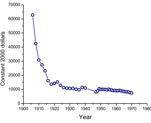
the second and third quintiles. The quality-adjusted price of new cars fell by 88 percent over the period
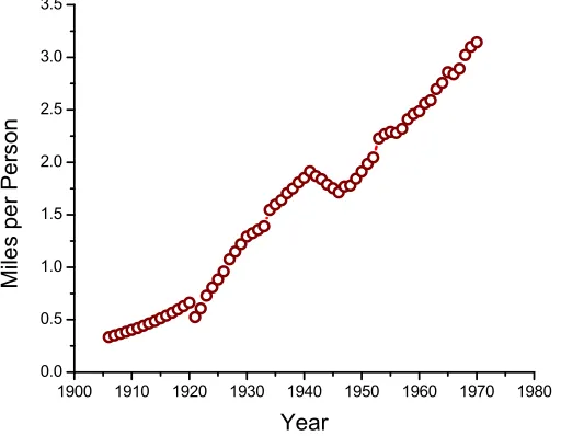
1906 to 1970 as shown in Figure 2.11
There is also a linkage between car-ownership and residential location. Figure 3 shows that families
living farther away from the city center are more likely to own cars than those living closer to the center
illustrating that households’ residential location choice and car-ownership decision are interrelated.
10
A detailed description of these data can be found in the data section of the appendix.
11 Source: Raff and Trajtenberg (1997). Their Table 2.9 shows the quality-adjusted price index for automobiles (in
1900 1910 1920 1930 1940 1950 1960 1970 1980 0
10000 20000 30000 40000 50000 60000 70000
C
o
n
s
t
a
n
t
2
0
0
0
d
o
l
l
a
r
s
[image:9.612.183.439.56.265.2]Year
Figure 2: Price of New Automobiles : 1906 - 1970. Source: See footnote 11.
1.3 The Analysis
The main objective of this study is two-fold: First, to quantify the importance of the diffusion of the
automobile in explaining postwar suburbanization. Second, to quantify the relative contributions of four
factors, namely rising real incomes, falling automobile prices, changes in transportation costs and urban
population growth, to suburbanization over the period 1910 to 1970. To achieve these, a variant of the
Alonso-Muth-Mills monocentric city model is developed.12 The model differs in three major ways from
the standard model. First, the model studied here allows for heterogeneity in household income. Hence
it is able to make predictions on the correlation between household income and residential location, and
the correlation between household income and car-ownership. Second, the current model incorporates
two modes of intra-urban transportation that differ in speed and costs: bus and car. The bus in the
model serves as a proxy for all forms of public transportation that are cheaper and slower than the
automobile. Finally, unlike the standard model which assumes that commuting is the only form of
intra-urban travel, the current study also allows for leisure travel. All non-commuting travel such as
travel for shopping, outdoor activities, and visiting friends or relatives is considered as leisure travel in
the model.
Households in the model economy have to choose a residential location and a mode of
transporta-tion. When agents make their location choices, they take into consideration three factors: the cost of
12 The time period in question justifies the use of monocentric city model. As mentioned in Section 1.1, the majority of
N o C a r O n e C a r T w o o r m o r e
0 -- 2 2 -- 4 4 -- 6 6 -- 8 10 -- 15 15 + 0 10 20 30 40 50 60 70 80 90 100 P e r c e n t o f G r o u p
[image:10.612.193.432.57.277.2]Distance f rom the City Center (m iles) Two or more One Car No Car
Figure 3: Car Ownership in 1962 by Distance from Center of Central City. Source: Survey of Consumer Finances, University of Michigan.
commuting, the cost of housing and the benefits of leisure travel. The desire to save on commuting
costs induces the households to live closer to the employment center. This in turn generates a large
demand for housing around the center and bids up rents. In the standard model, optimal location
choice involves a balance between these two forces. In the current study, however, the location decision
is also affected by a third factor: the benefits of leisure travel. Empirical evidence as well as everyday
experience shows that the density of stores, restaurants and people is higher in the central cities than
in the surrounding suburbs. Hence, when comparing to a suburban household, a household living close
to the city center does not have to travel as far from home for shopping, dining and other leisure
ac-tivities. This observation is captured in the model by allowing the benefit of traveling a fixed distance
for leisure to be decreasing in the distance from the city center. This provides an additional incentive
for city-dwellers to stay close to the center.
In the model, the choices of residential location and whether or not to purchase a car are closely
related. By owning a car, one can reduce the time costs of both commuting and leisure travel. This
induces households to spread to neighboring suburbs and enjoy larger living spaces. But not everyone
will choose to own a car. The price of a car serves as a fixed cost that screens out those with low
and this promotes suburbanization.13 Other features of the model that impact the rate of automobile
adoption and suburbanization are changes in the costs of traveling by car relative to bus and changes
in the size of the urban population. The importance of these factors in generating suburbanization is
assessed quantitatively as discussed below.
The model generates some interesting theoretical predictions on the spatial distribution of urban
populations. First, the model predicts a positive relationship between household income and distance
from the city center. In other words, poorer households in the model economy tend to locate closer to
the city center while wealthier households choose locations further away. This kind of spatial pattern
is consistent with empirical evidence. For example, according to the 1960 census, the median income
of households living in the central cities was 5,940 dollars compared to 6,707 dollars for suburban
households.14 It is also well-documented that a disproportionately large fraction of poor households in
the United States live close to the city center (Mills and Lubuele, 1997). Second, the model predicts
that bus-users and car-owners are segregated in terms of both income and residential location. More
specifically, there exists a unique threshold income level below which agents would choose to be
bus-users and live close to the city center, and above which agents would choose to be car-owners and locate
further away. Although such severe segregation is not observed in the real world, this result suggests
a close connection between public transportation usage and central city poverty which is supported by
empirical evidence. In a recent study, Glaeser, Kahn and Rappaport (2008) argue that better access
to public transportation in the central cities is an important factor in keeping low-income families in
such locations.
The model is solved numerically and calibrated to match data on car-ownership, suburbanization
over the period 1910 to 1940, as well as, travel times and commuting costs. Potential driving forces of
suburbanization and increasing car-ownership in the model are rising real wages, declining automobile
prices, an increase in the overall cost of using public transportation relative to using an automobile,
and urban population growth. All of which are taken either directly from the data or indirectly through
the calibration procedure. According to the model, the growth in urban population over the 1910 to
1970 period had only a small impact on car-ownership rates and suburbanization. The dominant driver
of suburbanization during the 1910 to 1950 period was declining prices of automobiles, followed by
13
Car price is assumed to be the only cost of purchasing a car. In particular, interest costs associated with credit financing are abstracted from. This abstraction is justified on two grounds. First, empirical evidence shows that most automobile purchasers did not use credit before 1950. Hence interest costs were a small fraction of ownership costs in the early years. Second, using existing data on the finance rate and the maturity of automobile credit for the period 1950 to 1970, it is estimated that interest costs are less than 10 percent of the price of a car. The actual percentage cannot be determined due to insufficient data. Details of these data are available upon request.
14
reductions in the time and fixed cost of traveling by car. However, from 1950 to 1970, rising real wages
played the dominant role, followed by the decrease in automobile prices. The impact of changes in the
time and fixed cost of traveling using public transportation was small. Under the baseline calibration,
the model is able to account for 60 percent of postwar suburbanization. The results support the
argument that basic economic forces such as rising incomes and falling transportation costs were the
primary drivers of suburbanization in the United States in both the prewar and postwar periods. In
addition, the results suggest that factors that are not considered in the model, such as “white flight” and
central city disamenities, may be important in explaining postwar suburbanization. These results are
thus consistent with Boustan (2007) which estimates that ”white flight” can explain about 20 percent
of the suburbanization trend between 1940 and 1970.15
This paper is closest in spirit to LeRoy and Sonstelie (1983). These authors extend the standard
monocentric city model by allowing for two modes of transportation. In their analysis, they provide
conditions under which the rich and the poor would choose different modes and live in different parts
of the city. Unlike the current study, LeRoy and Sonstelie did not explore the quantitative implications
of their model. They also assume that commuting is the only use of cars. Another paper which studies
suburbanization by extending the standard model is Baum-Snow (2007b). He extends the model by
adding highways which increase the speed of commuting. Similar to the standard model, the analysis
in his paper is based on a homogeneous population. It is thus unable to explain the correlation between
household income and residential location observed in the data.
The rest of this paper is organized as follows. Section 2 presents the model and the theoretical
results. Section 3 discusses the calibration procedure. Section 4 presents the baseline results and the
counterfactual experiments. This is followed by some concluding remarks in section 5.
2
The Model
2.1 The Environment
Consider a geographical regionP located on the Cartesian planeR2.Due to the existence of waterways
and other undevelopable geographical areas, real-world cities are rarely full circles. To capture this
15 Baum-Snow (2007a) is also closely related to the current study. For two reasons, however, it is difficult to compare the
60%
40%
Usable Land
CBD r
0
[image:13.612.248.386.47.173.2]2
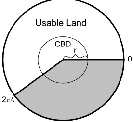
Figure 4: Schematic of Model City.
fact, it is assumed that only a portion of P is usable land that can consist of commercial, residential
and agricultural areas. At each distance s from the origin, a constant fraction Λ ∈ (0,1) of land is
assumed to be usable. Let C(s) denote the set of usable land at distance sfrom the origin. This can
be represented formally using polar coordinates. Letυ∈[0,2π] be a polar angle. Then C(s) is defined
as
C(s)≡ {(s, υ) :υ∈[0,2πΛ]}.
All usable land inP is identical and is uniformly distributed.
The model city is located on the usable part of P. An aerial map of the city is shown in Figure 4.
The size of the city is determined endogenously. The city has a single employment center called the
central business district (CBD). All production activities take place in the CBD. The CBD is centered
at the origin and is represented by B ≡ {C(s) :s∈[0, r]}.The radius r is set to (2πΛ)−1 so that the
total supply of usable land on the boundary of the CBD is normalized to one. All usable land outside
the CBD is rented for either residential or agricultural purpose in a competitive market.16 At each
distance x from the boundary of the CBD the total supply of usable land, i.e., land in C(x+r), is
given by 2πΛ (r+x).Each unit of land inC(x+r) is the same and, therefore, is let for the same rent
q(x). All rent is collected by a group of absentee landlords.
The city is part of a large economy in which there are two types of commodities: consumption
goods and automobiles. Both commodities are produced and traded within the city and in the larger
economy. Their prices are determined in the latter and taken as given by the inhabitants of the city.
There is a continuum of agents of mass N > 0 living inside the city. Each agent is characterized by
an ability λ∈[λmin, λmax].The ability distribution function is given byF(λ),with F(λmin) = 0 and
F(λmax) = N. All agents have to decide on a residential location which then serves as the point of
16
departure for all travel inside the city. There are two types of travel: commuting and leisure travel.
Since all the employment is located in the city center, all workers have to commute between their
residential locations and the boundary of the CBD for work. Travel within the CBD is assumed to be
negligible. All other traveling is classified as leisure travel. For any agent who lives in C(x+r),the
benefits of traveling a total distancez for leisure purpose is captured by
φ(x, z) =e−ηxzθ, withθ∈(0,1), η >0.
This specification satisfies the following assumptions regarding leisure travel. First, the benefit of leisure
travel is increasing in the total distance traveled since ∂φ(x, z)/∂z > 0 for all x, z > 0. Intuitively,
one can enjoy a wider variety of stores and recreational activities and visit more friends and relatives
by traveling a longer distance or taking more trips. However, there are diminishing returns to leisure
travel since 0< θ <1 implies that ∂2φ(x, z)/∂z2 <0 for all x, z >0. Second, for any given value of
z >0,the functionφ(x, z) is strictly decreasing inx.This feature is intended to capture the following
idea: since both businesses and people are more dispersed in the suburban areas, a person who lives in
the suburb (or further from the CBD) would have to travel a longer distance than one who lives in the
city (or closer to the CBD) in order to reap the same benefit from a leisure trip.
Each agent derives utility from consumption (c), residential land services (l) and the benefits of
leisure travel.17 The utility function is given by
U(c, l, z, x) =αlnc+ζlnl+ (1−α−ζ) lnφ(x, z),
whereα, ζ ∈(0,1).Each agent is endowed with one unit of time which can be divided between market
work, commuting and leisure travel.
There are two modes of transportation inside the city: bus and car. Bus services are available
throughout the entire city. These services are publicly owned and operated. On the other hand, any
agent who wants to travel by car has to buy one at pricepcand become a car-owner.18 An agent’s total
transportation cost is divided into two components: a time cost and a fixed cost. If the agent chooses
17
“Land” and “housing” are interchangeable in this paper. This implicitly assumes that the supply of housing is equivalent to the supply of land and is thus exogenously given. It also implies that the supply of housing is uniformly distributed throughout the urban area.
18
to travel a distancex by bus, then the total transportation cost is given by
t(wλ, x) =τb(x)wλ+γb, (2.2)
where w >0 is an exogenously given wage rate for an effective unit of labor, τb(x) is the amount of
time needed to travel the distancexby bus, andγb >0 is the fixed cost of using the bus. The function
τb(x) is assumed to be linear, i.e.,
τb(x) =ψbx, withψb >0.
The parameter ψb is the time required to travel a unit distance by bus. If the same agent chooses to
travel by car, then the total transportation cost is
τ(wλ, x) =τc(x)wλ+γc, (2.3)
whereτc(x) is the amount of time needed to travel the distance x by car, andγc>0 is the fixed cost
of using a car. The function τc(x) is given by19
τc(x) =ψcx, withψc>0.
The parameterψcis the time required to travel a unit distance by car. Notice that, conditional on the
mode of transportation, it is more costly for high-ability agents to travel than for low-ability agents.
Compared to taking the bus, the fixed cost of traveling by car is assumed to be higher, or
γc+pc> γb. (2.4)
However, it takes more time for bus-users to travel the same distance as car-owners, i.e.,
τc(x)< τb(x), for all x >0, (2.5)
or equivalently,ψc< ψb.
19
All the theoretical results in this paper remain valid when the time cost functionsτb(x) andτc(x) are generalized to
becomeτb(x) =ψbx σ andτ
c(x) =ψcx
σ,withψ
b>0, ψc>0 andσ >0.A complete set of proofs is available from
2.2 Bus-user’s Problem
Consider an agent with ability λwho chooses to do all his traveling by bus. Taking the rent function
q(·) and the market wage rate w as given, the agent chooses his consumption of goods (c) and land
services (l),time allocated to market work (m),the distance between his residence and the boundary
of the CBD (x) and the total distance to travel for leisure purposes (z) so as to maximize his utility
subject to his budget constraint and time constraint. Formally, the agent’s problem is given by
Vb(λ) = max
c,l,z,x,m{αlnc+ζlnl+ (1−α−ζ) lnφ(x, z)} (P1)
subject to
c+q(x)l+γb=wλm, (2.6)
m+τb(z) +τb(x) = 1, (2.7)
z, x≥0,
c≥0, l≥0, m∈[0,1].
Equations (2.6) and (2.7) are the budget constraint and the time constraint, respectively.
The problem (P1) can be solved in two steps. First, conditional on any distance x ≥0 such that
wλ[1−τb(x)]≥γb,the optimal expenditures on consumption goods and land, and the optimal amount
of time spent on leisure travel are determined by20
cb(λ, x) =eα[wλ(1−τb(x))−γb], (2.8)
q(x)lb(λ, x) =eζ[wλ(1−τb(x))−γb], (2.9)
and
wλτb(zb(λ, x)) =
³
1−αe−eζ´[wλ(1−τb(x))−γb], (2.10)
whereαe≡α/[α+ζ+ (1−α−ζ)θ] and eζ =ζeα/α.
The second step is to determine the optimal distance from the CBD. LetWb(λ, x) be the maximum
20 The use of logarithmic utility ensures thatc=l=z= 0 is never optimal. This also means it is never optimal to have
m= 0.The set of constraints can then be reduced to
c+q(x)l+wλτb(z) =wλ[1−τb(x)]−γb,
utility that a bus-user with ability λ can attain by choosing a location at distance x. This can be
obtained by substituting cb(λ, x), lb(λ, x) and zb(λ, x) into the utility function in (P1). The feasible
set ofx is given by
D(λ) ={x∈R+:wλ[1−τb(x)]≥γb}.
The agent’s optimal location choice, represented byxb(λ),is defined as21
xb(λ)≡arg max x∈D(λ)
n
Wb(λ, x)o. (P2)
The indirect utility function of a bus-user with abilityλis then given by
Vb(λ)≡Wb[λ, xb(λ)].
To illustrate the costs and benefits behind the choice of x, consider an agent with ability λwho is
comparing between two locations: one at distancex1≥0,the other at distancex2 > x1.The differences
inWb(λ, x) between these two locations can be decomposed into three parts:
Wb(λ, x2)−Wb(λ, x1)
= eθln
½
wλ[1−τb(x2)]−γb
wλ[1−τb(x1)]−γb
¾
−(1−α−ζ)η(x2−x1)−ζln
q(x2)
q(x1)
, (2.11)
where eθ ≡ α+ζ + (1−α−ζ)θ. By choosing to locate at x2 and hence live that much further away
from the CBD, the agent faces an increase in transportation costs and hence a reduction in net income
{wλ[1−τb(x)]−γb}.In response, the agent reduces consumption in goods and housing, and the time
spent on leisure travel. The loss in utility due to these reductions is captured by the first term in
(2.11). Moving away from the CBD would also lower the benefits of leisure travel. The loss in utility
due to this is captured by the second term in (2.11). If these losses are not checked by a decline in land
rent, then the agent would strictly prefer x1 tox2.In other words, if land rents are non-decreasing in
distance from the CBD then all the bus-users would choose to live as close to the CBD as possible. In
this case, the optimal location choice is xb(λ) = 0 for all λ. On the contrary, if an agent optimally
chooses to locate at distance x > 0, then it must be the case that q(x) < q(0) so that the costs of
21
Since τb(·) is continuous and strictly increasing, the feasible set D(λ) is a closed interval on the positive real line.
SinceWb(λ, x) is continuous inx,the optimal solution correspondencex
b(λ) is non-empty, compact-valued and upper
hemicontinuous inλ. In the following analysis, it is assumed that a unique solution for (P2) exists for all bus-users with abilityλ∈[λmin, λmax].In other words,xb(λ) is assumed to be a single-valued function for allλ∈[λmin, λmax].
Ifxb(λ) is single-valued and upper hemicontinuous, then it is a continuous function. The same uniqueness assumption
is made forxc(λ) defined in the car-owner’s problem. In the numerical analysis, caution is taken to ensure that the
moving away from the CBD are compensated by a reduction in rent.
One implication of this model is that, conditional on using the same mode of transportation,
high-ability agents choose to live further away from the CBD than low-high-ability agents. In other words, the
optimal location functionxb(λ) is an increasing function. This can be seen by considering (2.11) again.
As explained above, the first two terms in (2.11) capture the losses in utility when an agent moves
away from the CBD while the last term captures the gains in utility by doing so. Among these three
terms, only the first one depends on λ. In particular, this term is strictly increasing in λ.22 When an
agent moves further away from the CBD, less time is allocated to market work and hence net income
decreases. But the relative size of this reduction is not identical for all agents. Instead it is smaller for
high-ability agents than for low-ability ones. Thus, it is less costly for high-ability agents to move away
from the CBD. Consequently, bus-users with high ability would choose to live further away from the
CBD than those with low ability. This result is summarized in Lemma 1. All the proofs can be found
in the Appendix.
Lemma 1 The optimal location choice function for bus-users, xb(λ), is increasing over the range
[λmin, λmax].
2.3 Car-owner’s Problem
If an agent with abilityλ chooses to own a car, then he solves the following problem, taking the rent
functionq(·),the market wage rate wand the price of cars pc as given,
Vc(λ) = max
c,l,z,x,m{αlnc+ζlnl+ (1−α−ζ) lnφ(x, z)} (P3)
subject to
c+q(x)l+γc+pc=wλm,
m+τc(z) +τc(x) = 1,
z, x≥0,
c≥0, l≥0, m∈[0,1].
22
Mathematically, this implies that the functionWb(λ, x) satisfies strictly increasing differences in (λ, x).This property
Conditional on any distance x≥0 such thatwλ[1−τc(x)]≥γc+pc,the optimal expenditures on
consumption goods and land, and the optimal amount of time spent on leisure travel are determined
by
cc(λ, x) =αe[wλ(1−τc(x))−(γc+pc)], (2.12)
q(x)lc(λ, x) =eζ[wλ(1−τc(x))−(γc+pc)], (2.13)
and
wλτc(zc(λ, x)) =
³
1−αe−eζ´[wλ(1−τc(x))−(γc+pc)], (2.14)
LetWc(λ, x) be the maximum utility that a car-owner with abilityλcan attain by choosing a location
at distance x. The agent then chooses an optimal distance from the feasible set
{x∈R+ :wλ[1−τc(x)]≥γc+pc},
so as to maximize Wc(λ, x). Let x
c(λ) be the unique solution for this problem. The indirect utility
function for a car-owner with abilityλis then given byVc(λ)≡Wc[λ, x c(λ)].
Using the same proof as in Lemma 1, one can show that xc(λ) is an increasing function. This,
together with Lemma 1, implies that conditional on choosing the same mode of transportation,
high-ability agents will choose to live further from the CBD than low-high-ability agents.
Lemma 2 The optimal location choice function for car-users, xc(λ), is increasing over the range
[λmin, λmax].
2.4 Car-ownership and Location Decisions
An agent with ability λ will choose to own a car if and only if Vc(λ) > Vb(λ). The car-ownership
decision can be summarized by
Ω (λ) =
1, ifVc(λ)> Vb(λ),
0, ifVc(λ)≤Vb(λ),
(2.15)
forλ∈[λmin, λmax]. Define a critical ability levelλsuch that Vc
¡
λ¢=Vb¡λ¢.An agent with ability
λis indifferent between traveling by bus and purchasing a car for travel.
the city. The two groups of agents are said to be separated in terms of location if there exists x >0
such that one group of agents would live further than distancex from the boundary of the CBD while
the other group would live closer to the boundary thanx.In the current framework, assumptions (2.4)
and (2.5) are sufficient to ensure that car-owners and bus-users are separated in terms of location. This
result is summarized in Proposition 3.
Proposition 3 Suppose a critical ability level λ exists. Then there exists a unique pair of distances
(x,xe), x > xe ≥0, such that (i) all bus-users would live no further than distance x from the boundary
of the CBD, and (ii) all car-owners would live further than distancex but no further than ex.
2.5 Competitive Equilibrium
In the current context, a competitive equilibrium refers to a situation in which (i) competitive land
markets in every location clear and (ii) neither the agents nor the landlords have any incentive to
change their decisions. The following description focuses on an economy in which both car-owners and
bus-users exist. In the subsequent discussions, it is shown that at most one critical ability levelλexists
in equilibrium.
Equilibrium City Structure By Proposition 3, all agents will reside within distance xe from the boundary of the CBD. In other words, the city can be represented by
C={C(s) :s∈[0, r+ex]},
which includes the central business districtB={C(s) :s∈[0, r]}.In equilibrium, no usable land inP
is left vacant. Therefore all land in C\B must be utilized either for residence or for agriculture. If this
is not true then any rational landlord would lower the rent at the empty spot so as to induce someone
to move in. In fact, all land inC\B must be occupied by residence. This will become clear later on.
Since all agents are settled within the boundary of C, land beyond the city boundary is used for
agriculture. Let qA be the agricultural rent. The equilibrium rent function must satisfy
q(xe) =qA. (2.16)
rent out the land at distance xe to agricultural users. Suppose instead that q(xe) > qA. In this case,
agents living at distancexewould be strictly better off by moving to a location at distancexe+ε, with
ε > 0. If ε is sufficiently small, then the transportation costs and the benefits of leisure travel would
only be marginally affected but would be compensated for by a reduction in rent of q(ex)−qA. This
creates an incentive for those living at distance exto move and hence cannot be an equilibrium.
In equilibrium, all land in C\B is used for residential purposes. To see this, first defineR(x1, x2),
for any xe≥x2 > x1 ≥ 0,to be the set of usable land further than distance x1 from the boundary of
the CBD but no further than distancex2,i.e.,
R(x1, x2)≡ {C(s) :x1+r ≤s≤x2+r}.
Now suppose, to the contrary, that there exists some region R(x1, x2) inC\B that is used for
agricul-ture, while all other land in C\B is used for residential purposes. By the above argument, it must be
the case that q(x1) = qA. Since it is never optimal for any landlord to rent the land for less thanqA,
the rent charged to residents at distance x in (x2,x˜] must be q(x) ≥ qA. This means any agent who
chooses to locate at distancexin (x2,x˜] would be strictly better off by moving to a location at distance
x1 where the rent is the same or lower but the transportation costs are strictly lower and the benefits
of leisure trips are strictly higher. This creates an incentive for those who live in (x2,x˜] to move. Hence
this cannot be an equilibrium.
Car-ownership and Location In equilibrium, if a critical ability level λ exists then it must be unique. In addition, all agents with ability higher than λ will choose to own a car while those with
ability lower than λwill choose to use the bus. These results are summarized in Proposition 4.
Proposition 4 The following must be true in equilibrium:
(i) If a critical ability level λ exists then it must be unique. In additionxb
¡
λ¢=xc
¡
λ¢=x.
(ii) All agents with λ >(<)λwould choose to be car-owners (bus-users).
For any λ∈[λmin, λmax],define
The functionx(λ) summarizes the optimal location choice for every agent in the city. The next
propo-sition establishes that in equilibriumx(λ) is continuous and strictly increasing. Strict monotonicity of
x(λ) means that there is an one-to-one relationship between distance and ability. The city boundary
is then determined by
e
x=x(λmax) =xc(λmax).
Proposition 5 In equilibrium, x(λ) is continuous and strictly increasing over the range[λmin, λmax].
Equilibrium Rent Given a continuous distribution of abilities and continuous transportation cost functions for both car-owners and bus-users, it is immediate to see that the equilibrium rent function
q(x) must be continuous over the region where there are bus-users or car-owners only. This means
q(x) is continuous for any xgreater than or lower than x.Suppose q(x) is discontinuous atx and
q(x)> lim
x→x+q(x).
Given the gap in rent at distancex,any agent with critical ability levelλcan benefit by moving slightly
further out to a new location at distancex+ε > x.Sinceεcan be made arbitrarily small, a new location
can always be found such that the costs of moving there are over-compensated for by the reduction in
rent. This creates an incentive to move and hence cannot be a equilibrium. By a similar argument,
one can rule out the case with lim
x→x−q(x)> q(x).Hence q(x) is continuous over C.
Population Distribution For any distance yin [0,xe],let A(y)≡ {C(s) :r ≤s≤y+r}be the set of usable land that is no further than y from the boundary of the CBD. The population distribution
function,P(y),specifies the size of population living in the areaA(y) for anyyin [0,xe].The population
distribution function can be constructed using the optimal location choice functionx(λ),and the ability
distributionF(λ).To see this, first define the set Γ (y) by
Γ (y) ={λ∈[λmin, λmax] :x(λ)≤y},
for anyy in [0,xe].This set specifies the abilities of agents who optimally choose to live inA(y).Then
the population distribution function can be expressed as
P(y) =
Z
Γ(y)
withP(0) = 0 andP(ex) =N.
Competitive Land Markets In equilibrium, the demand for land by an agent with abilityλis given by
l(λ) =lb[xb(λ), λ] [1−Ω (λ)] +lc[xc(λ), λ] Ω (λ),
where Ω (λ) is defined in (2.15). For any distance y in [0,ex], the total supply of land in area A(y) is
given by
Λ
Z y
0
2π(r+x)dx= 2πΛry+ Λπy2,
where 2πΛr = 1 is the total supply of land on the boundary of the CBD. The land markets in area
A(y) clear if the total demand for land equals the total supply, or equivalently,
Z
Γ(y)
l(λ)dF(λ) =y+ Λπy2. (2.19)
Definition of Equilibrium Given an ability distribution F(λ),a competitive equilibrium of this economy consists of a set of decision rules for car-owners{cc(λ), lc(λ), zc(λ), xc(λ)},a set of decision
rules for bus-users{cb(λ), lb(λ), zb(λ), xb(λ)},a car-ownership decision rule Ω (λ),an optimal location
choice function x(λ), a population distribution function P(x), and a rent functionq(x) such that
1. Given the rent function q(x), for each bus-user with ability λ, the allocation {cb(λ), lb,(λ)
zb(λ), xb(λ)}solves (P1) and for each car-owner with abilityλthe allocation{cc(λ), lc(λ), zc(λ), xc(λ)}
solves (P3).
2. The car-ownership decision rule, Ω (λ),is given by (2.15).
3. The optimal location choice function,x(λ),is defined by (2.17).
4. The population distribution function, P(x),is given by (2.18).
5. The land market at every location clears, or (2.19) holds for all y ∈ [0,xe] and the rent at the
boundary of the city equals the agricultural rent, or (2.16) holds.
Characterization of Equilibrium The equilibrium defined above is made up of three parts: the bus-user’s problem, the car-owner’s problem and a critical ability level λ that connects the two. In
location choice functions for bus-users and car-owners are differentiable. The bus-user’s problem is
then characterized by a pair of differential equations:
x′b(λ) = wλf(λ) 1 + 2πΛxb(λ)
e
ζ
e
q(λ)
h
1−ψbxb(λ)−
γb wλ i , (2.20) and e
q′(λ) = −wλf(λ) 1 + 2πΛxb(λ)
½
ψb+
(1−α−ζ)η
e
θ
h
1−ψbxb(λ)−
γb
wλ
i¾
, (2.21)
whereqe(λ)≡q[xb(λ)] forλ∈
£
λmin, λ
¤
.The mathematical derivations of (2.20) and (2.21) are shown
in the Appendix. The optimal location function for bus-users must also satisfy the boundary conditions
xb(λmin) = 0 and xb
¡
λ¢=x.
Similarly, the car-owner’s problem is characterized by
x′c(λ) =
wλf(λ) 1 + 2πΛxc(λ)
eζ
e
q(λ)
·
1−ψcxc(λ)−
γc+pc
wλ
¸
,
and
e
q′(λ) = −wλf(λ) 1 + 2πΛxc(λ)
½
ψc+(1−α−ζ)η
eθ
·
1−ψcxc(λ)−
(γc+pc)
wλ
¸¾
,
whereeq(λ)≡q[xc(λ)] forλ∈
£
λ, λmax¤.The optimal location function for car-owners must satisfy the
boundary conditionxc
¡
λ¢=x, and the rent function that solves this system must satisfy the terminal
condition qe(λmax) =qA.
Finally, the critical ability level and the corresponding location are determined by the condition
Vb¡λ¢=Vc¡λ¢,which is equivalent to
η−1 + (ψb−ηψc)x=
η(γc+pc)−γb
wλ , (2.22)
where η≡(ψb/ψc)1−αe−eζ.Details on the numerical procedure used to compute the model equilibrium
can be found in the Appendix.
3
Calibration
In order to compute the model’s prediction for the contribution of automobile adoption to postwar
suburbanization a series of steady states is computed. The steady states represent an average
Table 3: Index of the number of urban households in the fifty largest cities in the U.S. in 1900.
Year 1910 1920 1930 1940 1950 1960 1970 No. of Urban Households 1.00 1.23 1.65 1.94 2.43 2.92 3.46
Source: See Number of Households in the Data Section of the Appendix.
of commuting, prices, population size, and the parameters governing the ability distribution will differ
across the steady states. Others such as the parameters governing preferences and the fraction of usable
land are assumed to be fixed. All parameters are pinned down using data. However some can be set a
priori while others must be determined by minimizing the distance between the model’s predictions for
a set of U.S. statistics to their counterparts from the data. The set of statistics targeted includes (i) the
mean population density gradients in the decennial years from 1910 to 1940 as estimated by Edmonston
(1975) and presented in Table 1, (ii) the percentage of households owning a car in the decennial years
1910, 1920, and 1950 through 1970 as shown in Table 2, and (iii) the fraction of total miles driven by
car-users for commuting to work in 1970. According to the National Personal Transportation Survey
conducted in 1969 this fraction was 0.37.23 Once the model parameters are chosen, the model’s
predic-tions on population density gradients for the period 1950 to 1970 are computed and the contribupredic-tions
of rising car-ownership to postwar suburbanization are quantified.
3.1 Parameter Values
Take the model period to be five years, which is close to the median age of passenger cars for the period
1950 to 1970.24 The following parameter values must be determined by the calibration exercise.
Usable Land The fraction of usable land in the city, Λ, is calibrated to 0.58 based on an estimate
reported in Hawley (1956). For a group of 157 metropolitan areas in 1940, Hawley finds that, on
average, the actual area of a city is only 58 percent of the area of the enclosing circle.
Number of Households Each agent in the model represents a single household. The number
of households in each decennial year t between 1910 and 1970 is denoted by Nt. Since Edmonston’s
estimates are for the forty-one largest U.S. metropolitan areas in 1900, a similar sample is constructed in
order to facilitate comparison. More specifically, a sample of the fifty most populous metropolitan areas
23
Source: National Personal Transportation Survey: Purposes of Automobile Trips and Travel, Report 10, May 1974.
24 The average median age of passenger cars in the U.S. over the period 1950 to 1970 was 5.1 years. Source: Ward’s
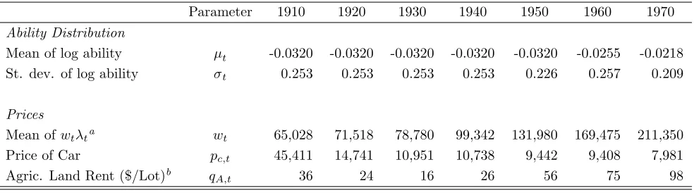
Table 4: The Evolution of the Ability Distribution, and Prices under the Baseline Calibration.
Parameter 1910 1920 1930 1940 1950 1960 1970
Ability Distribution
Mean of log ability µt -0.0320 -0.0320 -0.0320 -0.0320 -0.0320 -0.0255 -0.0218
St. dev. of log ability σt 0.253 0.253 0.253 0.253 0.226 0.257 0.209
Prices
Mean ofwtλta wt 65,028 71,518 78,780 99,342 131,980 169,475 211,350
Price of Car pc,t 45,411 14,741 10,951 10,738 9,442 9,408 7,981
Agric. Land Rent ($/Lot)b
qA,t 36 24 16 26 56 75 98
a
All prices are in constant 2000 dollars.
b
5-year rent. One lot is 12,910 square feet. (See footnote 26 for details.)
in 1900 is considered. These cities accounted for 75 percent and 57 percent of total urban population in
1910 and 1970, respectively. Since the total number of households in these cities are not known, a proxy
is constructed using the total population in these cities and the average size of nonfarm households in
the United States. Details of this approach are described in the Appendix. The resulting values of
{N1910,..., N1970} are reported in Table 3. The number of households increases at an average annual
rate of 2.1 percent over the period 1910 to 1970.
Preferences The parameters α and ζ determine the weights placed by households on utility from
consumption, housing services, and leisure travel. In the model economy there are three types of
consumption expenditures: consumption goods, housing services and transportation.25 Due to the
functional form for preferences, out of the first two categories, the share of expenditures on consumption
goods is given byα/(α+ζ). Thus the values ofαandζare chosen in the minimization procedure subject
to the constraint that this share matches the value observed in the data. Based on U.S. consumption
expenditure data reported in Lebergott (1996), on average, this share was 0.89 over the period 1910 to
1970. This requires α= 8.09ζ. The parameters determining the benefits of leisure travel,η and θ, are
determined by the minimization procedure.
Abilities In the model,wλis the maximum amount of earnings that a household with earning ability
λcan obtain by spending all its time endowment on work over a five-year period. The cross-sectional
variations inwλare driven by the variations inλacross households. For each decennial yeartbetween
1910 and 1970, the logarithm of λt is assumed to be normally distributed with meanµt and variance
25
σ2t.
Since there is no real-world counterpart forwtλt,its distribution is constructed using various sources
of data, including (i) average hourly earnings and employment across major industries over the period
1936 to 1970, (ii) time use data and (iii) labor-force participation rate among married women. Details of
this procedure can be found in the data appendix. Once the mean and variance ofwtλtare known, they
can be used to determine the values ofµt,σt, andwtunder the lognormal distribution assumption and
a normalization of the mean ability levels. Afterµtand σ2
t are determined, the lognormal distribution
is truncated so as to encompass 99 percent of the underlying population, omitting 0.5 percent from
each side. The values ofµt,σt, andwt at each datet are given in Table 4. Notice that wages increase
over the period generating a rise in real income in the model.
Agricultural Rent The rental rate of agricultural land, qA,t,is set to the rent paid for an average
single-family-sized lot of farmland at each date.26 The rental rate in each steady state is given in Table
4.
Car Prices and Transportation Costs Car prices between 1910 and 1970 are calibrated using
data on quality-adjusted prices reported in Raff and Trajtenberg (1997) [see footnote 11 for details]
and reported in Table 4.27 Car price for the steady state in 1910 is the average quality-adjusted price
over the period 1906 to 1910. The same rule applies to the other steady states. Notice that car prices
consistently fall over the 1910 to 1970 period.
In each steady state, there are four parameters governing the transportation costs, namelyγb,t, γc,t,
ψb,t,andψc,t.The parametersγb,t andγc,tcapture the fixed costs of using the bus and operating a car,
respectively. The time costs of using the two modes of transportation are determined byψb,t and ψc,t.
Unfortunately data on these costs for the time period in question are very scarce. Hence a number of
these parameters has to be determined by the minimization procedure.
26
The rental rate for an average single-family-sized lot of farmland is the gross rent paid for an acre of farmland divided by the number of average-sized lots in an acre. Data on gross rent are obtained from the U.S. Department of Agriculture Economic Research Service, the Census of Agriculture, theFarm Costs and Returns Survey, and theFarm Finance Survey. The number of average-sized lots in an acre is the average lot size for a single-family home taken from the National Association of Realtors.
27
1900 1910 1920 1930 1940 1950 1960 1970 1980 0.0
0.5 1.0 1.5 2.0 2.5 3.0 3.5
M
ile
s p
e
r
P
e
r
so
n
[image:28.612.186.442.62.261.2]Year
Figure 5: Miles of Paved Urban Road per Urban Population : 1906 - 1970. Source: See footnote 30.
Automobile In the model, the parameter ψc is the time required to travel one unit distance by car. One possible way of calibrating this is to exploit travel time data for car-users. This kind
of data, however, is very scarce for the period in question. The only data source available is the
National Personal Transportation Survey conducted in 1969. According to this study, the average time
to commute one mile by car was 3.63 minutes in 1970.28 When translated to model units, this means
ψc,1970 = 0.0054.29
For the other decennial years, the time cost of traveling by car is assumed to be a function of the
availability and quality of roads, measured by the total mileage of paved urban roads per 1,000 urban
population. Figure 5 plots the time series of this measure over the period 1906 to 1970.30 Throughout
this time period, the total mileage of paved urban roads per 1,000 urban population rose at an average
annual rate of about 3.5 percent. For each decennial yeartfrom 1910 to 1960 letRtdenote the average
total mileage over the t−4 tot period. The time cost is then assumed to be the decreasing function
of Rt,
ψc,t= ΦR−tκ.
The parameters Φ andκ are chosen through the minimization procedure subject to the constraint that
28 Source: Authors’ calculations based on the data reported in Table A20 in
National Personal Transportation Survey: Home-to-Work Trips and Travel Report No. 8, August 1973.
29 Consider a car-owner who has to take a roundtrip between home and work each day for five days a week. The total
time spent on commuting is 3.63×2×5 = 36.3 minutes per week. Assume that the agent is awake for 16 hours a day. The total amount of time available is 16×60×7 = 6,720 minutes per week. The parameterψc,tatt= 1970 is given
by 36.3/6,720 = 0.0054. 30
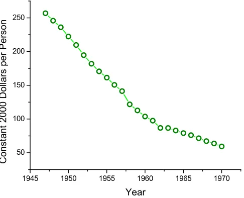
1945 1950 1955 1960 1965 1970 50 100 150 200 250 C o n s t a n t 2 0 0 0 D o l l a r s p e r P e r s o n Year
Figure 6: Capital Stock of Equipment and Structures for Intercity and Local Passenger Transit per Urban Population, 1947-1970. Source: Fixed Reproducible Tangible Wealth in the United States, 1925-70.
ψc,1970 = 0.0054.
The fixed costs of traveling by car are calibrated using data on car-related consumption expenditures
reported in Lebergott (1996). The data include expenditures on tires and accessories, gasoline, oil,
repairs, automobile insurance and tolls. The fixed costs parameterγc,tis equated to the five-year total
expenditures per registered vehicle.31 The costs are given in Table 8. The fixed costs decrease from
approximately 14 (constant 2000) dollars in 1910 to 5.42 dollars in 1970.
Bus The efficiency of many forms of public transportation such as streetcars and motor buses also depends on the quantity and quality of roads per person. Thus, the time cost of commuting by bus
is assumed to be a function of both the quantity of paved urban roads per urban person and the value
of equipment and structures in public transit per urban person. Figure 6 shows the value of the stock
of equipment and structures per urban person for intercity and local passenger transit over the period
1947 to 1970. The value is a measure of both the quantity and the quality of the pubic transit stock.
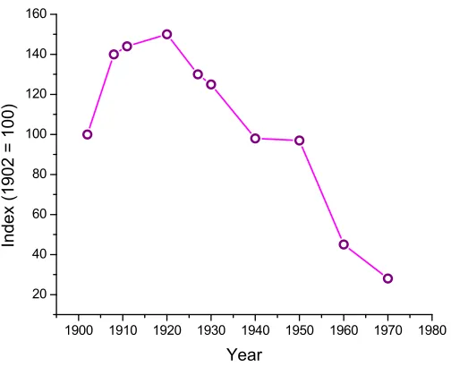
The value declined steadily over this time period at an annual rate of 6 percent. Evidence shows that
the decline in public transit began much earlier than 1947. First, public transit ridership per capita
has been persistently declining since the 1920’s as shown in Figure 7. Second, net capital expenditures
on transit equipment and structures were negative for the period 1920 to 1950 (see Table 5). This
31
1900 1910 1920 1930 1940 1950 1960 1970 1980 20
40 60 80 100 120 140 160
I
n
d
e
x
(
1
9
0
2
=
1
0
0
)
[image:30.612.187.439.56.261.2]Year
Figure 7: Public Transit Ridership per Capita, 1902-1970. Source: Jones (1985).
suggests that the public transit sector has been disinvesting since the 1920’s. Given this evidence, it
seems reasonable to assume that the capital stock in public transit has been declining since, at least,
1930. On the one hand, this decline suggests of decrease in services, which should raise the time costs of
using public transit by lengthening waiting times and increasing the distances between stops. However,
on the other hand, the increasing quantity and quality of roads should make certain forms of public
transit such as buses more efficient, reducing time costs. Which of these two effects dominates will
come out of the minimization procedure.
The ideas mentioned above are captured formally as follows. Let Pt denote the t−4 tot five-year
average of the stock of equipment and structures in public transit per urban person. For the decennial
years between 1930 and 1970, the time cost parameter for bus is assumed to be
ψb,t= ΓRtρ−1Pt−ρ, (3.23)
where Rt is the total mileage of paved urban roads per 1,000 urban population as defined above. The
parameters Γ and ρ are chosen through the minimization procedure. For the years 1926 to 1947 Pt
is estimated using a linear trend. The trend is not extended to the years before 1926 because it is
questionable whether the capital stock was declining during these early years. Instead it is assumed
thatψb,tis growing at a constant rate prior 1930 so that
ψb,t= Ψ (g)
t−1910
The parameters Ψ andgare again determined by the minimization procedure subject to the constraint
thatψb,1930 is the same whether obtained by (3.23) or (3.24).
The fixed costs of traveling by bus are calibrated using U.S. consumption expenditure data on local
public transit over the period 1900 to 1970 taken from Lebergott (1996). The values ofγb,tare obtained
by dividing the total expenditures on local public transit overt−4 to tby the number of households
without cars. The costs are given in Table 7. The fixed costs, for the most part, increase over the 1910
to 1970 period from 1.81 (constant 2000) dollars in 1910 to 4.26 dollars in 1970.
3.2 Minimization Procedure
Ten parameters are still undetermined up to this point. These include the preference parameters: α
and ζ, the parameters governing the benefits of leisure travel: η and θ, the time cost parameters for
automobile: Φ and κ, and the time cost parameters for bus: Γ, ρ, Ψ, and g. Let θ denote the vector
of unknown parameters. In the minimization procedure, the vector θ is chosen so as to minimize the
discrepancies between the model’s predictions and the observed data. The choice of θ is subject to
three constraints. First, the preference parametersαandζ are chosen so that the share of expenditures
on consumption goods matches the data. This requires
α= 8.09ζ. (3.25)
Second, the time cost parameters for automobile (Φ and κ) are chosen so that the predicted value of
ψc,1970 is consistent with the average time spent on traveling one mile by car observed in the data. This
requires
ψc,1970= ΦR−1970κ = 0.0054. (3.26)
Third, the time cost parameters for bus are chosen so that the value of ψb,1930 as predicted by (3.23)
is consistent with that predicted by (3.24). This means
ΓRρ1930−1P1930−ρ = Ψ (g)19301910−1910. (3.27)
After taking into account these constraints, seven degrees of freedom remain. These are chosen to
match ten targets: (i) the mean population density gradients for each decennial year between 1910
and 1940, (ii) the percentage of car-owners in each decennial year between 1910 and 1970 (excluding
Table 5: Net Capital Expenditures of Urban Transit Properties, 1890-1950.
Year 1890 1900 1910 1920 1930 1940 1950 Net Expendituresa 74.0 170.9 66.1 -128.5 -82.3 -10.4 -53.5
amillions of 1929 dollars. Source: Ulmer (1960).
commuting in 1970. At each datet, denote the model’s prediction on the percentage of car-ownership
byVt(θ),the population density gradient byDt(θ),and the fraction of total miles driven by car-users
for commuting byMt(θ). To compute the population density gradient, the population density at 1,000
locations in [0,xet] is computed. Let{xi,t}and {yi,t} be the set of locations and the sample population
densities, respectively. The population density gradientDt(θ) is obtained from the following regression:
lnyi,t =At+Dt(θ) lnxi,t+εt. (3.28)
In all the experiments below, the R-square of (3.28) is always greater than 0.8. The fraction of total
miles driven by car-users for commuting is given by
Mt(θ) =
R
xc,t(λ;θ) Ωt(λ;θ)dF(λ)
R
[xc,t(λ;θ) +zc,t(λ;θ)] Ωt(λ;θ)dF(λ)
,
where Ωt(λ;θ) is the indicator function defined in (2.15).
In the minimization procedure,θ is chosen so as to minimize the sum of the deviations between the
model’s output and the observed data, subject to the three constraints described above. Formally, letvt
denote the actual percentage of car-ownership in the U.S. at timet,dtbe the actual population density
gradient for an average American city and m1970 be the fraction of total miles driven by car-users for
commuting in 1970. Thenθ is chosen by solving
min
θ
( 1920
X
t=1910
[vt−Vt(θ)]2+
1970X
t=1950
[vt−Vt(θ)]2+
1940X
t=1910
[dt−Dt(θ)]2+ [m1970−M1970(θ)]2
)
,
subject to (3.25) through (3.27). The parameter values determined by the minimization procedure are