Available online www.jocpr.com
Journal of Chemical and Pharmaceutical Research, 2014, 6(5): 608-616
Research Article
CODEN(USA) : JCPRC5
ISSN : 0975-7384
Content and Eigenvector Centrality-Based Music Classification Algorithm
Xin Wang
Computer Engineering School, Weifang University, Shandong 261061, P. R. China
ABSTRACT
With the rapid development of Internet and the improvement of the storage techniques, more and more music resources are gotten, and correspondingly their classification becomes an important issue. Up to now, three main classification methods have been proposed, which are Tag-based approach, content-based approach and the methods based on machine learning. Although these approaches have been analyzed and compared based on the music features; there are still no deep researches on the intrinsic relationship between the music. This paper focuses on this issue and presents a novel music classification algorithm based on both the music content and the critical eigenvector centrality. Firstly, the new algorithm extracts the MFCC (Mel Frequency Cepstrum Coefficient) and Rhythm features of music, and then the K-Means algorithm is used to cluster these features. As a result, K-cluster centers are generated. Correspondingly, the music network using similarity relations can be constructed. At last, the music network is analyzed by using a graph-based eigenvector centrality and the music classification is completed by joint considering the K-cluster centers. Moreover, experiments are provided to evaluate the new proposed classification algorithm, and its performance is also compared with the conventional content-based classification algorithm. The results show that the new music classification algorithm is more reasonable to satisfy the needs of most of users.
Key words:
Content
;
Eigenvector centrality
;
K-Means algorithm
;
Music Classification
INTRODUCTION
With the rapid development of information technology and the huge improvement of people life, getting music from internet has become an important part of usual life. Furthermore, a large number of excellent internet musical works continue to emerge and spread with the development of the Internet, the acceleration of music creation cycle, and the improvement of music compression and storage techniques. And then, how to manage more and more musical resources becomes an important issue. In this area, many kinds of analysis methods have been proposed and investigated in details in order to discover the potential rule and pattern hidden in the music.
______________________________________________________________________________
609
machine learning proposed by Shlomo, Dubnov in [1]. Where, they used the neural network machine learning method to learn the music samples, analyzed the mapping relationship between musical features and corresponding classification, forecasted and classified the new music after mastering classification rules. In order to construct the connection between music and emotion, some researchers have developed the music analysis methods based on both content and emotion. Human emotions have been classified by Kerstin Bischoff, which contained a variety of emotion categories. And then, through the analysis of music content the corresponding features could be extracted, and the different musical categories could be mapped to the corresponding emotions. Consequently, each piece of music has a corresponding emotion expression, which was really convenient for users to understand the meaning of the music.
As mentioned above, many scholars have proposed a variety of solutions for music classification; however, these methods only used one or several characteristics of the music as the basis for analysis and classification, and still lacked attention and analysis on the intrinsic relationship hidden in the music. As a result, the accuracy and reasonableness of classification will become another problem [2]. To solve this problem, this paper proposes a novel music classification algorithm based on the music content and the eigenvector centrality, and the design goal is to make the classification results more satisfy the user's appreciation.
RELATED WORKS
Yu-Lung Lo proposed the content-based music classification method [3], in which they extracted a variety of musical features used in classification. However, this method is not much accurate to solve the question of single music feature classification. Jianhui Liu et al. proposed instrument classification method based on least squares support vector machine [4], where they extracted the MFCC and other music features. By combining with LS-SVM theory the classification of different instruments could be achieved, and the accurate rate was up to 90%. Carlos N. and Silla Jr. [5] used genetic algorithm (GA) to optimize the selection and combination of the music characteristics, and the accuracy of the classification could be further improved. Matthew Hoffman et al. worked more in-depth. In [6] they used a non-parametric Bayesian model HDP (Hierarchical Dirichlet Process) to further mine the potential structure characteristics of MFCCs, and the similarity in the color of music could be analyzed.
NOVEL MUSIC CLASSIFICATION ALGORITHM
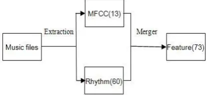
The novel music classification algorithm concludes the following four steps. a) Firstly, extract two kinds of music features, which are MFCC and Rhythm.
b) Secondly, determine the numbers to be classified. These features are clustered to calculate all music, and to obtain the feature center of each category.
c) Thirdly, via using Euclidean distance calculate the similar relationship between each pair of music. In order to generate music network, independent music is interconnected to form a network.
d) Finally, calculate the category of music by using the eigenvector centrality, and complete the music classification.
A. Music Features Extraction
Digital music can be roughly divided into lossy and lossless music according to the sound quality. The lossy music has a certain percentage compression and filtering of the original music files, which is small for easy storage and transmission. But the sound quality will have more or less loss inevitably, and it is unable to retain all the characteristics of the music. Lossless music is not compressed, and contains every detail of the music. So it has completely perfect sound quality. However, its file size is proportional to its mass, as a result a large storage is required and not conducive to upload and download.
Xin Wang
J. Chem. Pharm. Res., 2014, 6(5): 608-616
______________________________________________________________________________
music.
[image:3.595.211.418.136.231.2]In this paper, the two features are extracted by using the third-party music feature extraction tool named as MARSYAS. By this way each piece of music is represented by a final 73-dimensional vector. Extraction and combination of music features are shown in Figure 1.
Fig. 1. Extraction and combination of music features
In order to extract the two music features, two third-party libraries are also adopted [8]. One is Audio Feature Extraction [9], and the other is MARSYAS (Music Analysis,Retrieval and Synthesis for Audio Signals) [10]. Audio Feature Extraction is developed and maintained by institute of software technology and interactive systems technology of Vienna University, which supports music feature extraction under both Windows and Linux platforms. By using the Audio Feature Extraction, the user can easily get the Rhythm characteristics of the music. MARSYAS is another open source C++ based software framework for music processing, which is mainly used for music information extraction. MARSYAS is jointly developed by Professor George Tzanetakis of Victoria University of Canada, his students, and researchers from around the world, which is a mature tool for music information extraction, and widely used in many projects of industry and scientific research in academia. MARSYAS is powerful, while supporting Windows, Mac OS and Linux development platforms, can extract Timbre, Chroma, Pitch, MFCC, SNR and other music features.
By using MARSYAS and Audio Feature Extraction based on the Linux (Fedora) platform, combined with QT development environment, this paper completes the final work of music information extraction, which includes two kinds of music features, which are MFCC and Rhythm. Eventually, each extracted piece of music forms a 73-dimensional vector. In addition, in order to make rational use of resources, and to deliver more music information to the users, MARSYAS is also used to extract some common label information, including name, music album, artist, genre, theme and broadcast time, etc.
Music features are commonly used in music analysis, music management and recommendation algorithms. A common operation is to calculate the distance between the music features, compare the characteristics of a piece of music with another, and analyze the similarity relationship. Assuming the number of music in a library is n, you need a total of n n( 1) / 2 times in comparison to calculate the similarity relationship between each pair of music. Although this paper only selects two kinds of music features as the basis for analysis, the 73-dimensional feature vector will have still a greater effect on the analysis efficiency.
B. Select the Cluster Center
For the classification of a large-scale music library, this paper firstly determines the number of specific types of categories, and further determines the representative music in each class, i.e. the clustering center. The center represents the type of music.
In this paper K-Means clustering algorithm is used to calculate the clustering center [11]. K-means is a very typical clustering method based on distance, in which the distance is used as the similarity evaluation index. I.e. the closer the two objects, the greater the similarity. The algorithm considers a cluster containing the objects with the closer distance, so the compact and independent object distribution becomes the ultimate goal.
In the K-means algorithm, the first step is to specify a cluster granularity parameter denoted by K and the corresponding cluster centers. The center selection of the K initial clusters has significant influence on the clustering results. Usually, K random objects are selected as the initial cluster centers, and each center represents a cluster. And then, the remaining objects of the dataset are traversed, and each object will be re-allocated to the nearest class according to the distance from the cluster center.
______________________________________________________________________________
algorithm has converged or the operation has reached a specified number of iterations. In the iteration, it will indicate that the algorithm has converged when each cluster center has not changed in the iterative process.
After the feature extraction, each piece of music is represented by a 73-dimensional vector. According to the theory of K-means algorithm, all music in the music library can be calculated by the following steps to achieve clustering and get the cluster centers.
a) Set the clustering granularity parameter K, which is the number of classification. b) Randomly select K clustering centers from the corresponding objects.
c) Calculate the distance of the remaining objects from each cluster center, and put it into the nearest class. d) Recalculate the cluster center of each class.
e) Do iteration from c) to d) until the clustering centers no longer change or the iterative operation has reached the specified maximum number of iterations.
f) The clustering results are saved to the corresponding objects.
The above algorithm can implement the clustering of each feature component.
C. Establishment of Music Network
The new classification algorithm is graph-based, which is mainly to determine which piece of music is the most important in a music library. In details, the algorithm involves two aspects. One is the establishment of a graph-based network based on the musical features and their relationship between them. The other is to calculate the importance of the music based on the graph-based network by using the analytical methods.
The music network is the basis of the graph-based analysis algorithms. Here, each node of the music network represents a piece of music, and the weight of each edge of the music network denotes a similar relationship between the corresponding music nodes. In the following, by taking the extracted music features into account, the music network establishing method is proposed on the basis of the Euclidean distance and the maximum spanning tree algorithm.
a) Initialize the music network.
The main initializing operation is to calculate the relationship between each pair of music. And the calculation is based on the previously extracted characteristics, which are MFCC and Rhythm. In this paper, the Euclidean distance [12] is adopted for the relationship distance calculation. For each pair of music, the closer the distance, the greater the similarity.
Suppose that a music library contains n songs, and each one contains m features. And the features of the i-th music are represented by Fi=( Fi[1], Fi[2], Fi[3],…Fi[m]), 1 i n. s(i, j) denotes the similarity relationship between the i-th and j-th music, which is calculated as follows.
2 1
1
( , ) ,1
1 ( [ ] [ ])
m
i j
k
s i j k m
F k F k
(1)
The music network is described by the above distance relationship. In which, each node represents a piece of music, while each edge between pair of nodes will be assigned a weight to indicate the similarity, which is the calculated distance. Because each weight ranges from 0 to 1, it is actually an undirected complete graph.
b) Generate an initial maximum spanning tree.
The scale of the current music network is really too large to be calculated. In fact, in a music network only the edges with the larger weight will have significant effect on the results of the recommendation algorithms, while the others with the lower weight do not play an important role. In order to improve the efficiency of the calculation, in this paper the recommendation algorithm tends to focus on the larger weight edges only. In another words, the maximum spanning tree algorithm is adopted for reduction and optimization of the complete graph with retaining only a few larger weight edges, which results in a simplified music network.
Xin Wang
J. Chem. Pharm. Res., 2014, 6(5): 608-616
______________________________________________________________________________
weighted graph network containing n vertexes; the corresponding spanning tree has only (n-1) edges
The most widely used spanning tree is the minimum spanning tree, in which, the weight of the spanning tree is equal to the sum of the weights related to all edges in the connected graph network. The minimum spanning tree has an important significance for the daily life and work, which is usually used in the calculation of minimum cost in order to help resource conservation. However, in this paper, the analysis tends to focus on the edges with lager weights only, just for the purpose of improving efficiency while maintaining good sound quality as much as possible. It is based on the fact that only the lager weights represent the most obvious similarity for the music relationships, which also has an important contribution to the recommended algorithm. Therefore, the maximum spanning tree is used in this paper instead of the minimum spanning tree. Referring to the definition of the minimum spanning tree, the maximum spanning tree can be defined as: For a weighted connected graph, the weight of the maximum spanning tree is equal to the sum of the larger weights of the related edges.
Currently, there are two main maximum spanning tree generation algorithms. One is Prim algorithm [13] and the other is Kruskal algorithm [14]. Here, the Prim generation algorithm is adopted to generate the corresponding maximum spanning tree, which includes the following steps.
(1) Given a new vertex set S and a set of edges TE, the initial state of S and TE are empty.
(2) Randomly select a vertex K from the current generated undirected music network diagram. Construct the maximum spanning tree from K, and add K to S.
(3) Select the edge with the maximum weight denoted by (X,Y), XS, YS. (4) The edge (X, Y) was added to TE. And Vertex Y joins the set S.
(5) Repeat (3) and (4) operation until the n-1 edges are selected. (6) Get the maximum spanning tree T= (S, TE).
With the above algorithm, the corresponding maximum spanning tree could be generated from an undirected weighted music network. The new generated spanning tree only contains n music nodes and n-1 edges; as a result, the music network could be greatly simplified.
c) Generate the second maximum spanning tree.
In the previous step, the maximum spanning tree algorithm is used to simplify the original music network, but this maximum spanning tree still can not meet the final needs. In fact, music network has two functions. One reflects the similarity relationship, and the other is to describe the importance of each piece of music in the network. The generated initial maximum spanning tree contains only n-1 edges, which can only reflect some important similarity relationship, but can not be conducive to describe the importance of the node. In order to solve this problem, this paper constructs the second maximum spanning tree, which includes two main steps. Firstly, a new network infrastructure is produced by removing the edges for the initial maximum spanning tree from the complete graph; secondly, an additional maximum spanning tree is generated from the new produced network. The detailed process is described as follows.
(1) Let G = (V, E) be an undirected complete weighted graph. And T= (S, TE) is the initial maximum spanning tree generated from G. By removing the edges of initial maximum tree T from the complete graph G, a new network is produced denoted by G '= (V, E-TE).
(2) Based on the new produced network G ', do the same operation as the initial maximum spanning tree, a second maximum spanning tree T '(S', TE ') could be generated. The biggest difference compared to the initial spanning tree is that the initial maximum spanning tree generated based on the complete graph, while the second maximum spanning tree is generated in the new produced network by removing n-1 edges.
d) Generate the final music network.
The final music network is generated by combining the initial maximum spanning tree T and the secondary maximum spanning tree T '.
As mentioned above, only one maximum spanning tree is too simple to meet all the needs of recommendation algorithm. It is necessary for one music network to provide sufficient information for the recommendation system, while to maintain their simplicity and efficiency. One possible way is to merge the two maximum spanning trees, and create a new network. Jointly considering the initial maximum spanning tree T and the secondary maximum spanning tree T ' could provide a more important similarity relationship, and they can provide important reference for the recommendation algorithm. In other words, the new network is relatively simple, which contains only 2n-2 edges, while it is more accurate to describe the relationship between the music.
D. Music Classification Based on Eigenvector Centrality
______________________________________________________________________________
will be assigned to each node according to the quantity and quality of edges connecting to this node. The range of this value determines the importance of this node in the network, and hence it is named as eigenvector centrality. In other words, the importance of a node in the network is determined by the number and the weight of the edges connected to this node. According to this definition, connecting a small number of high quality (high weight) nodes is more important than the connection of a plurality of low weight nodes, and the network location is closer to the "center". Obviously, it is more scientific and reasonable via using a network analysis method based on eigenvector centrality, which can reveal deep-seated nature of the information network.
Centrality measure is one of the most basic and common network structure analysis methods, which aims to find the most important node in a network. Which node is the most important one? There may be a variety of answers largely depending on how to understand the word "important". Undoubtedly, the degree provides a very simple way to do the centrality measure. According to the definition, the degree of a node indicates the number of edges connected to this node in the network, which is reasonable and effective for measuring the influence or importance of a node in the whole network. For example, in a social network, if a person contacts more partners, more resources could be got from it. In another words, it has more importance than others. Of course, the degree only provides one of the understandings to the word "important", for other understandings, different results will be produced. Currently, the most commonly used centrality calculation methods include Closeness Centrality, Betweenness Centrality, Eigenvector Centrality, and so on [15].
Closeness centrality is generally used in the undirected graph, which describes the connection state of a node in the graph, and the state can explain the distance or closeness of a node from others. For one node in the graph, its closeness centrality is represented by the average shortest distance, which is obtained by averaging the sum of all the shortest paths’ length from this node to every other node in the network. In general, for one node the smaller closeness centrality indicates the closer relationship between this node and others. Such node with smaller closeness centrality is usually located in the center of the whole network. Thus, there is sufficient reason to believe that the cost of communication between such node and others is lower and its importance is becoming bigger correspondingly. Of course, a contrary view also exists, where it is believed that the larger value of a node’s closeness centrality indicates its more important role playing in the network. As for what kind of point of view is adopted, it really depends on the network environment and the actual requirement.
Obviously, a node’s closeness centrality needs to calculate the shortest path between the node and every other node. However, the shortest path may not exist for some pair of nodes, just because they are not reachable. For such cases, a common solution is to ignore these infeasible paths, while only to calculate the shortest reachable paths. The closeness centrality is calculated as follows.
1
( , )
( ) ,
n i j j
i
d v v c v j i
m
(2)Where, n denotes the total number of nodes in the network, c v( )i represents the value of the closeness centrality of
node vi, d v v( ,i j) accounts for the shortest path between nodes vi and vj, and m represents the number of all
reachable shortest paths. From (2) it can be seen that the final results of the closeness centrality are only affected by the network structure, i.e., the path information, while has nothing to do with the weights of node itself and edges. Betweenness centrality is another method to measure the importance of a node in a graph, which has different meaning from the former closeness centrality. In fact, closeness centrality represents the relationship of distance, while betweenness centrality represents the dependency among the nodes. In other words, one node’s betweenness centrality accounts for the degree that other nodes in the network are dependent on this node. Obviously, if the majority of nodes in the network have to rely on a node, the node will play an important role in the network. In other words, if this important node is ineffective, it will have a great impact on the structure of the whole network and the interconnected relationship between each pair of nodes. And hereby “between” can be used to reflect the network's dependence of multiple nodes on one node, which is the main idea of betweenness centrality. In order to calculate the betweenness centrality of the nodes in the network, the shortest paths between any pair of nodes in the network should be firstly achieved. And then the betweenness centrality of the node v could be calculated as the ratio of the shortest paths through node v to all the shortest paths between any pair of nodes in the network. Specifically, the betweenness centrality of the node v could be described as follows.
( ) ( )
st s v t
st s v t
d v b v
d
(3)Xin Wang
J. Chem. Pharm. Res., 2014, 6(5): 608-616
______________________________________________________________________________
which passes through the node v. Obviously, dst( )v has two values. When the shortest path between
s
and tcontains the node v, dst( )v will be equal to one. Otherwise, it has no meaning and will be set to be zero.
The shortest path has important significance for a network, which generally represents the minimum cost or the shortest distance. It is clear that one node will occupy an important position in the network if it frequently appears in these shortest paths between each pair of nodes. Once the node does not exist, a large area of "circuit breaker" may be caused, or the shortest distance of the entire network will have a huge change. It has proved that betweenness centrality is a relatively simple and direct approach to calculate the importance of each node in many social networks, however, only using this metric is not sufficient to fully express the importance of a node. In some cases, the node with high betweenness centrality may not be the central node of the network. The reason is that betweenness centrality does not consider the weights of the nodes and edges.
Different from closeness centrality and betweenness centrality, eigenvector centrality is a more mature network analysis method. Compared to the two former centrality calculation methods, eigenvector centrality can provide more and deeper information, in which the network nodes and edges are considered in a different way. Specifically, the importance degree connecting an important node should be higher than that connecting multiple non-significant nodes. Inspired by this idea, the eigenvector centrality approach assigns each node an importance degree according to the quantity and quality of edges connecting to it. And the value of the importance degree will determine the importance of this node in the network. In other words, the importance of a node in the network is determined by the number and the weight of the edges connecting to it. According to this definition, the node with a small number of high quality (high weights) edges will be more important than the node with a plurality of low weight edges, and it will be closer to the "center" of the network. Obviously, it is more scientific and reasonable by using eigenvector centrality, which can express deep-seated nature information of the network. Currently, this method has been used in various networks [16]. Moreover, the well-known search engine “Google” also uses eigenvector centrality on the Webpage sorting.
For the K cluster centers successfully selected before, the eigenvector of each piece of music is used to compare and select K corresponding music. Next, the corresponding K nodes are identified in the established music network. For other music in the library in addition to the selected K music, their critical eigenvectors are also calculated one by one relative to the K nodes, and the calculation steps are expressed as follows.
Firstly, define the following variables:
A: Denote the adjacency matrix of the music network with each element representing the connection state between the corresponding nodes.
ij
A
: Denote the element of the matrix A, which represents the connection strength (weight) between node i and
node j. Aij 0 means that there is no connection between these two nodes.
n: Denote the number of nodes in the music network, or the number of music in the music library.
i
x : Denote the eigenvector centrality of the i-th node.
x : Denote the eigenvector of matrix A corresponding to the eigenvalue , which is expressed as
1 2
( ,x x ,... )xn
x
.
Next, the critical eigenvector is calculated for each piece of music corresponding to the node i, which includes a) Measurement calculation of the initial eigenvector center for the input music node i.
According to the principle and idea of the eigenvector, the centrality metric xi of node i can be calculated as
1
1
. n
i ij j
j
x A x
(4)
In which is a constant, which represents a proportion. xj denotes the importance of the neighbor nodes. From
(4), it can be seen that the importance of node i is decided by connection strength Aij between the node i and
its neighbor nodes. And hence, 1
x Ax (5)
x Ax (6)
______________________________________________________________________________
b) For the music node j j, i in the network, delete all edges associated with it, and generate a new matrix denoted by A.
c) Calculate the eigenvectors x via using (6), and get the eigenvector centrality xi.
d) Calculate the critical change c i j( , ) xi xi corresponding to node i, which is caused by deleting the edges of
a node j, so c i j( , ) is the eigenvector of node j relative to node i.
e) Repeat the steps from (b) to (d) for the entire music network, and get the eigenvector of the entire music nodes according to the target node, denoted by c i j( , ),1 j n i, j.
Through the above algorithm, the eigenvector of each music node in music network can be calculated with respect to the K nodes. And then, by putting each node to the corresponding cluster according to the sequence of critical eigenvector key, and the music classification for the entire music library could be achieved.
EXPERIMENTS
In this part, a set of experiments is provided to compare the new proposed music classification algorithm and the conventional content-based music classification algorithms. From which the advantages of the new algorithm will be further demonstrated.
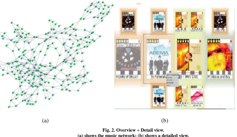
Moreover, the Overview+Detail visual interface and interaction techniques are developed to facilitate the users to validate the algorithm. As shown in figure 2, the designed view is divided into two parts. The music network structure is shown in figure 2 (a), in which each node represents a piece of music, and each edge between nodes represents the similarity relationship between music. The global view, i.e., Overview is demonstrated in the part of the figure 2 (b), which displays all the music in the user’s local music library.
Through the music network and Overview, a lot of music can be shown in a limited space. When a user is interested in a particular piece of music, the node is clicked and the music is displayed in the Detail view. At the same time, the designed algorithm helps users to obtain the similar music. In other words, when users in the Detail view click one music, new focus and related recommendation are constantly created, and the whole music classification and recommendation are continued.
[image:8.595.81.481.433.663.2](a) (b)
Fig. 2. Overview + Detail view.
(a) shows the music network; (b) shows a detailed view.
Here, music classification is reasonable and not directly related to the user's experience. The classification results for different users are different. Therefore, in this paper the algorithm is tested and evaluated by using the user survey.
Xin Wang
J. Chem. Pharm. Res., 2014, 6(5): 608-616
______________________________________________________________________________
points, while the lowest score is 0 points. Experimental results show that the averaged scores for the traditional content-based classification algorithm and the new designed classification algorithm are 6.5 and 7.3, respectively, which demonstrated that the new proposed music classification algorithm is more humanized and reasonable.
CONCLUSION
This paper proposes a new music classification algorithm based on both music content and critical eigenvectors. In which, two kinds of music features are jointly considered, which are MFCC and Rhythm. Compared with the conventional content-based classification algorithms, the new one can further improve the classification accuracy, and help to satisfy the user's appreciation and enjoy the preference. This result has been clearly proved by the practical experiments. Furthermore, the new designed method could produce a simple music network and it is significant for the efficient management of large music resources, even for large data system.
REFERENCES
[1]K. Bischoff; C. S. Firan; R. Paiu; and W. Nejdl. Music mood and theme classification-a hybrid approach, 10th International Society for Music Information Retrieval Conference (ISMIR 2009), pp. 657-662, 2009.
[2]T. Lei, Content and user history-based music visual analysis.Shandong University, 2012.
[3]Y. L. Lo, Content-based music classification, 3rd IEEE International Conference on Computer Science and Information Technology (ICCSIT), pp. 2-6, 2010.
[4]J. Liu; L. Zeng. Instrumental music classification based on least squares support vector machine, Journal of East China Jiaotong University, vol. 26, no. 6, pp. 60-64, 2009.
[5]C. S. Jr; A. Koerich. Improving automatic music genre classification with hybrid content-based feature vectors,
Proceedings of the 2010 ACM Symposium on Applied Computing, pp. 1702-1707, 2010.
[6]M. Hoffman; D. Blei. Content-based musical similarity computation using the hierarchical dirichlet process,
Proc.Int.Conf.Music Information Retrieval, pp. 349-354, 2008.
[7]S. Baumann. Music similarity analysis in P2P environment, Proceedings of the 4th European Workshop on Image Analysis for Multimedia Interactive Services, no. 3, pp. 1-7, 2003.
[8]R. Typke; F. Wiering. A survey of music information retrieval systems, Proc.Int.Conf.Music Inf.Retrieval(ISMIR), pp. 153-160, 2005.
[9]G. Tzanetakis. MARSYAS submissions to MIREX 2009, Proceedings of the Music Information Retrieval, 2009.
[10]K. A. A. Nazeer. Improving the accuracy and efficiency of the k-means clustering algorithm, Proceedings of the World Congress on Engineering, vol. 1, pp. 1-5, 2009.
[11]L. Sarmento; F. Gouyon. Music artist tag propagation with wikipedia abstracts, ECIR-WIRSN, 2009.
[12]P. Danielsson. Computer graphics and image processing, vol. 14, no. 3, pp. 227-248, Nov. 1980.
[13]R. C. Prinl. Bell system technical journal, vol. 36, pp. 1389-1401, 1957.
[14]T. L. Maganti; J. B. Orlin. Network Flows: Theory, Algorithms, and Applications. Prentice-Hall, Englewood Cliffs, 1993.
[15]L. Ding; F. Yu; S. Peng; C. Xu. Journal of Computers, vol. 8, no. 8, pp. 2077-2083, Apr. 2013.