Diffraction Problem in Radar Level Gauge Verification
Peter Mikuš
*, René Harťanský, Oľga Čičáková
Institute of electrical engineering, Faculty of Electrical Engineering and Information Technology, Slovak University of Technology in Bratislava, Bratislava, Slovakia
*Corresponding Author: [email protected]
Copyright © 2014 Horizon Research Publishing All rights reserved.
Abstract
This article deals with verification of radar sensors. Although these are very accurate devices, they are vulnerable to distortion of the measured value due to false reflections. Since this is an assigned measure, it must be ensured that results are fixed and reproducible. This places the onus on geometric and environmental optimalization to minimize false reflections and deliver accurate measurements.K
eywords
Radar Level Gauge, Verification, Reflections, High-Frequency Wave, Diffraction
1. Introduction
The radar level gauge is a device which measures distance using an indirect method without contact. The radar sensor uses continuous frequency modulation and consists of two basic integrated parts: a transmitter and a receiver. The transmitter is a signal generator with directional antenna, while the receiver comprises a directional antenna, an amplifier, a decoding device, a circuit with the voltage comparator and a powerline circuit. The latest sensors are non-sensitive to temperature, pressure and density changes and also to the composition of the gas in the measuring environment.
The continuous frequency modulated system
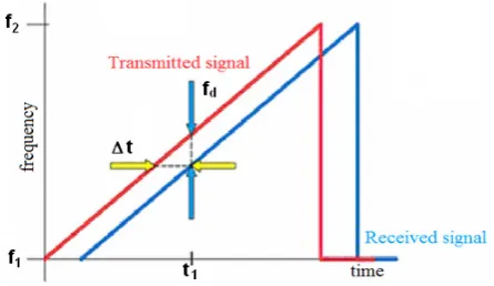
Most current level sensors work through continuous frequency modulation, using measurement of the difference in transmitter and receiver frequencies. The transmitted frequency is swept between two known values f1 and f2, and
the distinction between the transmitted signal and the return signal is measured as in Figure 1. [2]
Verification of level gauges
Verification takes place in the Department for verification of radar sensors, located in the long corridor on the ground floor of the SLM n.o .building. Fixed beams under the 2.2 m. ceiling of the corridor hold the metal guide rail.
A reflection board simulating the water level in the tank moves on the metal bar via a toothed belt and servo drive. A large rack is situated at one end of the hall. This holds the calibrated level gauge 1.35 m above the floor and the etalon
[image:1.595.323.546.334.463.2]of the length - the laser interferometer XL 80. Disturbances can occur in this method of verification. For example, disturbance reflections appear unless adequate space is available. The maximum radiation angle of the level meter is 13 °, the width of the corridor is 1.93 m and the beams are 0.85 m distant. From this, we can calculate parasitic reflections [3]
Figure 1. The principle of "continuous frequency-modulated signal"
m
46
,
7
5
,
6
85
,
0
=
=
=
⇒
=
tg
tg
d
x
x
d
tg
α
α
(1)where: d = distance from the ceiling
Our verification conditions give beam reflections at approximately 7 metres, and therefore distorted measured values at distances over 7 m. Since we can not change the environment we solve this problem by focusing a ray which avoids reflection from the walls. One solution is to build an anechoic wall which absorbs electromagnetic waves before parasitic reflection can occur. The next problem is to provide an upright reflection board towards the level gauge. When this is insufficiently upright, it causes distinction between the rays floating to the top and bottom parts of the board, and therefore distance measurement error occurs. The shape, location and edges of the board affect the extension of the radar waves, and thus level gauge accuracy verification.
Figure 2. Undesired reflections in level gauge verification
2.
Scattering by Steel Beams
Cylinders form one of the most essential classes of geometrical surfaces, and they compose the surface of many practical scatters including aeroplane fuselages and missiles. The circular cylinder is geometrically simple and is easily solved by tabulated functions such as those of Bessel and Hankel, and it is studied in detail here because it is used very widely in practical scatters..This especially involves scattering of both plane and cylindrical waves by circular conducting cylinders of infinite length at normal and oblique incidences, and the solutions herein are obtained using modal techniques. Scattering from finite length cylinders is derived from transformation of infinite length scattered fields using approximate relationships.
2.1. Plane Wave Scattering by Conducting Circular Cylinder: TM polarization
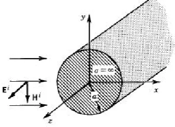
When it is assumed that a TM uniform plane wave is normally incident on a perfectly conducting circular cylinder of radius a, as in figure 3.
Figure 3. Uniform plane wave incident on conducting circular cylinder, TM polarization
then, the electric field can be written as;
ϕ cos 0 0
ˆ
ˆ
ˆ
jkr z jkx z i z zi
a
E
a
E
e
a
E
e
E
=
=
−=
− (2)However, equation (2) is inappropriate for further solution of the scattered field, as it is transformed into an appropriate form for derivation of the diffraction on the cylindrical structure. Here, we use Bessel functions of the Fourier series. The complex coefficients of the Fourier series have the form j-n. , so that;
( )
∑
∞ −∞ = −=
n jn n nz
E
j
J
kr
e
a
ϕ0 i
ˆ
E
(3)or
( )
j
ε
J
( ) ( )
kr
n
ϕ
E
a
E
i=
ˆ
z 0−
n n ncos
(4)where
≠
=
=
0
,
2
0
,1
n
n
nε
(5)The total electric field around the conductive cylinder is;
s i
t
E
E
E
=
+
(6) where; Esis the scattered field. Since the scattered fields travel in an outward direction, they are expressed by cylindrical travelling wave functions, so that Es is;( )
∑
∞ −∞ ==
=
n n n
z s z z
s
a
E
a
E
c
H
kr
E
(2)0
ˆ
ˆ
(7)Similar to the situation in the Fourier series’s approximation of incidental fields, here cn defines the
unknown amplitude coefficients. Equation 7 has similar form to Equation (4), and the combination of these two defines the total field. This then aids solution of cn amplitude
coefficients which are determined by applying the boundary condition, as;
(
,
0
2
,
)
0
ˆ
=
≤
≤
=
=
a
E
r
a
z
E
tz z
t
ϕ
π
(8)Combining (4), (7), and (8) then derives
(
)
( )
( )( )
[
]
∑
∞ −∞ = −+
=
=
=
≤
≤
=
n n n
jn n n t z
ka
H
c
e
ka
J
j
E
z
a
r
E
0
,
2
0
,
2 0 ϕπ
ϕ
(9) or( )
( )
( )
jnϕn n n n
e
ka
H
ka
J
j
c
=
−
− 2(10)
Thus the scattered field of (7) reduces to
( )
( )( )
( )( )
∑
∞ −∞ = −−
=
n jn n n n n sz
E
j
H
J
ka
ka
H
kr
e
E
2 ϕ [image:2.595.89.268.473.602.2]( )
( )
( )
( )( ) ( )
∑
∞=
−
−
=
0
2 2
0
(
)
cos
n n n
n n
n
H
kr
n
ka
H
ka
J
j
E
ε
ϕ
(11)where; εn is defined by (5).
3. Problem Formulation
[image:3.595.379.554.85.285.2]Our problem centres on the department which verifies radar level gauges depicted in Figure 4.
Figure 4. Department verifying radar level gauges
A significant increase in measurement error develops in verification level gauges at distances longer than approximately 7 m. Equation (1) determined that the electromagnetic waves focused from the level gauge onto the steal beams at exactly 7.45m, created diffractions and distortion around the beams. Therefore the shape of the final field around the radiated beams calculated in Figure 5 presents the geometry required to solve our problem.
Figure 5. Geometry of the solved problem
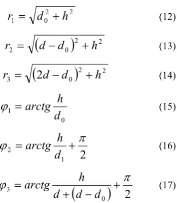
This is achieved by calculating the electric field from the three beams at distances r1, r2, r3 from point P and rotated by
angles ϕ1, ϕ2, ϕ3 to plane x. The distance between the beams is d = 500 mm and the observation plane is at distance h = 950 mm from the beams. The observation point P is moved in 5 mm steps from the border of the first beam to the border of the last beam. The distances of relevant points r1, r2,
r3 are calculated by Equations (12), (13) and (14) and the
angles ϕ1, ϕ2, ϕ3 are calculated as in Equations (15), (16) and
(17).
2 2 0
1
d
h
r
=
+
(12)(
)
2 2 02
d
d
h
r
=
−
+
(13)(
)
2 20
3
2
d
d
h
r
=
−
+
(14)0 1
=
arctg
d
h
ϕ
(15)2
1 2
π
ϕ
=
+
d
h
arctg
(16)(
0)
2
3
π
ϕ
+
−
+
=
d
d
d
h
arctg
(17)Equation (11) provides diffraction electic fields E1(r1, θ, ϕ1), E2(r2, θ, ϕ2), E3(r3, θ, ϕ3) at observation point P, and
defines the total diffraction field, thus;
3 2
1
E
E
E
E
s=
+
+
(18)To determine the total electric field at the observation point, it is necessary to calculate the incidental primary electric field Ei (ρ, θ, ϕ) according to formula (3), where the
distance r = ρ. Here, ρ defines the distance of the point from the actual start of this system, and therefore from the level gauge antenna.This is clearly illustrated in Figure 6.
Figure 6. Illustration of distance ρ
The resultant total electric field at observation point P is determined by Formula (6).
4. Results
[image:3.595.67.288.206.369.2] [image:3.595.64.293.499.619.2]define the total field. These graphs are identical to those featured in worldwide literature [1].
[image:4.595.327.539.156.291.2]Figure 7. The diffraction field surrounding one beam
Figure 8. The total electric field surrounding one beam
The analytical calculation of the problem formulated in section 3 required development of an algorithm for step by step alteration of observation point P’s position in the direction of the x-axis in ρ to ρ + d intervals. The distances r1, r2, r3 for each selected point P are calculated by Equations
(12), (13) and (14) and ϕ1, ϕ2, ϕ3 angles by Equations (15),
(16) and (17). These values are used to calculate diffraction fields from each beam, and their summation determines the total diffraction field at point P. Figure 9 depicts the scattering field calculation performed without considering the phase shift in the difraction fields of each beam, while
Figure 10 allows for delayed formation of the diffraction fields. The scattering fields from each beam do not arise simultaneously; these depend on the time of the impact of the incidental wave. The first beam radiates initially, then the second and finally the third, and this phenomenon is included in the initial phase of each beam’s scattering field.
Figure 9. The course of the scattering electric field under the beams - without considering the phase shift of the beams
Figure 10. The course of the scattering electric field under the beams- considering the phase shift of the beams
The sum of the diffraction fields and the incidental field is shown in Figure 11. This elucidates the distribution of the electric field under the beams along the measuring department.
Precise complex and demanding computations allow a clear picture of what is happening in the beam’s fields when they are irradiated with the radar signal from the level gauge.
[image:4.595.325.537.329.465.2] [image:4.595.63.289.373.592.2] [image:4.595.326.538.592.729.2]Figure 11 shows significant inhomogeneity in the electric field along the measuring department, thus influencing a calibration uncertainty in the radar level gauges which is more than coincidental in this case. This graph highlights the measuring department’s inappropriate layout and the need to alter its design to minimize diffractions on the beams and to prevent results such as the ones so clearly illustrated in the graph.
5. Conclusion
Verification of radar level gauges requires measurements performed with minimum error.When these instruments are used for very precise measurements, such as the fuel level in large tanks, a measurement error of 1 mm creates a vast difference in volume. Since the maximum measurement error allowed is + / - 0.5 mm, these instruments must be verified annually to detect any source of error. Although several sources of error exist in the verification environment, this article concentrates on the influence that the steel beams exert on the emitted radar waves. Because the radar level gauges operate at 10 GHz frequency and 30 mm wavelength, the resultant wave is widely spread, and when the radius of the beams was compared to wavelength, no simplified calculation for electric field distribution was adequate.
To verify the precision of the demanding calculations thus required, we first established the field around the beam and compared our results to those in the literature [1]. These corresponded; ensuring that our calculations were correct. We then applied this principle to multiple beams, as described in section 3. It was essential to establish the electric field under the beams because the reflection board which simulates water level is situated in close proximity. Figure 9 shows the calculated course of the electric field under the beams. It is evident that this field was highly inhomogeneous due to the presence of the steel beams. These
combined circumstances effected distance measurement errors which grossly devalued the level gauges verification
Acknowledgement
s
This work was supported by the Slovak Research and Development Agency under contract No. APVV-0333-11- “Electromagnetic compatibility of technology in rubber industry” and VEGA project No. 1/0963/12 “Validation methods of selected test of EMC”.
REFERENCES
[1] Balanis, A., C.: Advanced Enginnering Electromagnetics, John Wiley & Sons, New York, 1989
[2] Mikuš, P., Harťanský, R., Problems with Reflections of Radar Wave Consider the Radar Level Gauge. In ELITECH´13: 15th Conference of Doctoral Students; Bratislava, Slovakia, 5 June 2013. Bratislava: Nakladateľstvo STU, 2013, s. 4. ISBN 978-80-227-3947-4.
[3] Mikuš, P., Harťanský, R., The Errors in Radar Level Gauge Calibration. In Measurement 2013 : Proceedings of the 9th International Conference on Measurement. Smolenice, Slovakia, May 27-30, 2013. Bratislava: Slovak Academy of Sciences, 2013, s. 355--358. ISBN 978-80-969672-5-4. [4] Bittera, M., Kamenský, M., Smieško, V.: Broadband
Antennas Scanning Error as Contribution to Uncertainty of EMI Measurement. In: Measurement 2013 : proceedings of the 9th international conference on measurement. Smolenice, Slovakia, May 27-30, 2013. - Bratislava : VEDA, 2013, pp. 351-354