and Diffusing Surfaces in Auditoria
by
Trevor John Cox
This thesis was submitted for the degree of Doctor of Philosophy in the Department of Applied Acoustics, University of Salford.
Page
1 2 9
Contents
Contents
Table of illustrations Acknowledgements Abstract
Glossary of symbols
Chapter L Introduction
1.1 Introduction
1.2 Objective Measurements 1.3 Subjective Measurements
Chapter 2. The Measurement of Scattering from Finite
Sized surfaces
2.1 Introduction 12
,
2.2 Possible Methods to Measure Sound Scattering 12
2.2.1 Directional microphone method 13
2.2.2 Impulse source system 14
2.2.3 Time delay spectroscopy 16
2.2.4 Doublet source method 17
2.2.5 Cross correlation methods 17
2.2.6 Summary of methods available 18
2.3 Two Microphone, White Noise Source, Cross Correlation 20 System
2.3.1 General principle of measurement system 20 2.3.2 The theoretical basis for the cross correlation method 25 2.3.3 Separation of incident sound and reflected sound 28
2.3.4 Microphone calibration 32
2.3.5 Movement of the diffuser microphone 32
2.3.6 Assessment of measurement accuracy 35
2.3.7 The problem with using white noise 40
2.4 One Microphone, Pseudo-random Noise Source, Cross 40 Correlation Method
2.5 Reasons for Measuring the Scattered and Total Field 44
2.6 Displaying of Results 45
Reflectors and Diffusers
3.1 Introduction 47
3.2 The Helmholtz-Kirchhoff Integral Equation 47 3.2.1 Definition of the Helmholtz-Kirchhoff integral equation 47
3.2.2 Local reacting admittance assumption 49
3.3 General Solution Method 50
3.4 3D Boundary Integral Method 51
3.5 Solution of the Integral Equation in the Thin Panel Limit 53
3.6 Transient Model 57
3.7 Kirchhoff Approximate Solution 58
3.8 Fresnel and Fraunhofer Approximate Solutions 59
3.8.1 Solution for rigid plane panels 61
3.8.2 Solution for non-rigid surface 63
3.9 Geometric Approximation to Curved Panel Scattering 64
3.10 Conclusions 65
Chapter
4.
Theoretical Predictions and Measurements of the
Scattering from Thin Rigid Plane Panels
4.1 Introduction 67
4.2 The Panels Tested and the Measurement System Used 68
4.2.1 The panel measured 68
4.2.2 Measurement system used 68
4.2.3 Other panel tested 68
4.3 Theoretical Predictions Methods 69
4.4 Results and Discussions 69
4.4.1 3D Boundary integral method 69
4.4.2 Thin panel limit solution 72
4.4.3 Kirchhoff approximate solution 76
4.4.4 Fresnel solution 80
4.4.5 Fraunhofer solution 81
4.5 The Cut-off Frequency for Plane Reflectors 88
Chapter 5. Theoretical Predictions and Measurements of the
Scattering from Curved Panels
5.1 Introduction 97
5.2 The Panels Tested and Measurement Technique 98
5.2.1 The curved panel measured 98
5.2.2 The measurement system used 98
5.2.3 Other curved panels tested 98
5.3 Theoretical Prediction Methods Used 99
5.4 Results and Discussions 100
5.4.1 3D boundary integral method 100
5.4.2 Thin panel limit solution 100
5.4.3 Kirchhoff approximate solution 145
5.4.4 Geometric scattering theories 105
5.5 The Cut-off Frequency for Curved Panels 112
5.6 Conclusions 114
Chapter 6. Theoretical Predictions and Measurements of the
Scattering from Quadratic Residue Diffusors
6.1 Introduction 116
6.2 A Brief Introduction to Quadratic Residue Diffusers 117 6.3 The Diffusers used for Measurements and Predictions 122
6.3.1 The QRD used for measurements 122
6.3.2 A simplified constant depth diffuser 123
6.3.3 Other QRD models 125
6.4 Theoretical Models used for QRD and CDD 126
6.4.1 Thin panel limit solution 126
6.4.2 Representing of the QRD by a box of variable admittance 127
6.4.3 3D boundary integral method 129
6.4.4 Kirchhoff approximation 129
6.4.5 Simple Fraunhofer solution 129
6.4.6 Other methods 130
6.5.4 High frequency prediction techniques 134 6.6 Measurements and Predictions of a QRD 140
6.6.1 Thin panel limit solution 140
6.6.2 3D boundary integral method 144
6.7 Simulated Quadratic Residue Diffusers 147
6.7.1 Cut-off frequency 148
6.7.2 Lower frequency limit 153
6.7.3 Kirchhoff approximate solution 153
6.7.4 Simple Fraunliofer theory 160
6.7.5 Comparison of computation time for theories 163
6.8 Conclusions 165
Chapter 7. The Relative Performance of Diffusing and
Reflecting Surfaces
7.1 Introduction 169
7.2 The Scattering Performance of Quadratic Residue Diffusers 170
7.2.1 'Optimum' diffusion 170
7.2.2 QRD Performance compared to Fraunhofer solution 172 7.2.3 QRD performance compared to uniform scattering 178 7.2.4 Performance of a QRD with an oblique source 178 7.3 The Relative Performance of Diffusers and Reflectors 183 7.3.1 Scenario for comparing diffusers and reflectors 183
7.3.2 Normal incidence case 184
7.3.3 Oblique incidence 187
7.4 Conclusions 190
Chapter 8. The Subjective Measurement System
8.1 Introduction 192
8.2 Experimental Systems for Subjective Testing 193
8.3 The Simulator 198
8.4 Reflection Sequence Used in the Tests 200
8.4.3 Balancing lateral to non-lateral energy 206
8.4.4 Reverberation simulation 211
8.4.5 Clarity index, centre time and deutlichkeit 212
8.4.6 Overall sound level 218
8.4.7 The impulse response 218
8.5 Motifs Used in the Tests 219
8.6 Setting Up Procedure 220
8.7 Test Subjects 222
8.8 Test Method 222
8.8.1 Overview of methods available 222
8.8.2 Method of minimal changes 225
8.9 Analysis Techniques 226
8.9.1 Testing for training and fatigue, the F test 226
8.9.2 Calculating the limen 228
8.10 Conclusions 228
Chapter 9. The Difference Limen for Spatial Impression
9.1 Introduction 229
9.2 Experimental Method 229
9.3 Results for Handel Motif 231
9.4 Results for Mendelssohn Motif 232
9.5 Effects of Motif 233
9.6 Difference Limen for Early Lateral Energy Fraction 234 9.6.1 Figure of eight microphone measurement 235
9.6.2 Direct calculation 236
9.6.3 Results 237
9.7 The Difference Limen for Inter Aural Cross Correlation 238 Coefficient
9.7.1 Definition of IACC 238
9.7.2 Calculation of IACC 240
9.8 Comparison with Previous Measurements 241
Chapter 10. The Difference Limen of Clarity
10.1 Introduction 245
10.2 Experimental Method 246
10.3 Objective Parameters Used for Clarity 248
10.4 Results 250
10.4.1 Results for Handel motif 250
10.4.2 Results for Mendelssolm motif 251
10.4.3 Comparison of results for the two motifs 251
10.5 Comparison With Previous Results 252
10.6 The Difference Limen for Clarity Index 256 10.7 Discussion of Difference Limen Results for Spatial Impression 257
and Clarity
10.8 Conclusions 259
Chapter 11. The Perception of Diffuse Reflections in
the Sound Field
11.1 Introduction 260
11.2 Simulation of Diffuse Reflections 260
11.3 Measurement Technique 265
11.4 Results and Discussions 266
11.4.1 Spatial effects 266
11.4.2 Frequency differences 267
11.5 Conclusions 268
Chapter 12. The Initial Time Delay Gap
12.1 Introduction 269
12.2 Experimental method 270
12.3 Results and Discussions 271
12.3.1 Lateral reflection results 271
12.3.2 Ceiling reflection 273
12.3.3 Discussion 274
12.4 Comparison with Previous Measurements 274
12.4.2 Measurements by Ando 276
12.5 Conclusions 277
Chapter 13. Conclusions
13.1 Introduction 279
13.2 Objective Measurements 279
133 A General Result from Theoretical Predictions 280 13.4 Results for Plane panels and Curved Panels 280
13.4.1 Results common to both panels 280
13.4.2 Results applicable to plane panel only 281 13.4.3 Results applicable to curved panels only 282
13.4.4 The use of a cut-off frequency 283
13.5 Results and Discussions for Quadratic Residue Diffusers 284 133.1 Guidelines to predicting the scattering from QRDs 285 13.6 Performance of Diffusers and Reflectors 286
13.7 Subjective Measurements 287
13.7.1 Difference limen for spatial impression 288
13.7.2 Difference limen for clarity 288
13.7.3 Discussions of difference limen results 288
13.7.4 Diffuse reflection tests 289
13.73 The initial time delay gap 289
13.8 Conclusions 290
Chapter 14. Further Work
14.1 Development of Theoretical Prediction Methods 291 14.2 Optimization of the Quadratic Residue Diffuser 292
14.3 Further Subjective Work 293
14.3.1 Improving the subjective measurement system 293
14.3.2 Further subjective measurements 294
Appendix 1. Error Calculation for Two Microphone
296Measurement System
page
Plate 1.1 Quadratic residue diffusers in situ in a recently built 7 concert hall.
Plate 1.2 End view of a quadratic residue diffuser in a recently 8 built concert hall.
Plate 2.1 The set up within the anechoic chamber for the 34 measurement of scattering from diffusers and reflectors.
Plate 6.1 The quadratic residue diffuser measured. 119 Plate 8.1 The loudspeakers in the anechoic chamber in the 205
subjective measurement system.
Acknowledgements
Abstract
The performance of reflectors and diffusers used in auditoria have been evaluated both objectively and subjectively.
Two accurate systems have been developed to measure the scattering from surfaces via the cross correlation function. These have been used to measure the scattering from plane panels, curved panels and quadratic residue diffusers (QRDs). The scattering measurements have been used to test theoretical prediction methods based on the Helmholtz-Kirchhoff integral equation. Accurate prediction methods were found for all surfaces tested. The limitations of the more approximate methods have been defined. The assumptions behind Schroeder's design of the QRD have been tested and the local reacting admittance assumption found to be valid over a wide frequency range. It was found that the QRD only produces uniform scattering at low frequencies. For an on-axis source the scattering from a curved panel was as good as from a QRD. For an oblique source the QRD produced much more uniform scattering than the curved panel.
Glossary of Symbols
a Half panel width
Speed of sound
Cso Clarity index
C(a) Cosine part of Fresnel integral Cxy Real part of cross spectrum
or C'(w) Real part of processed cross spectrum
Cxyi or C1 (6)) Real part of cross spectrum for measurement with the diffuser
Cxy2 or C2(w) Real part of cross spectrum for measurement without diffuser Difference between minimum and maximum path lengths from panel to receiver
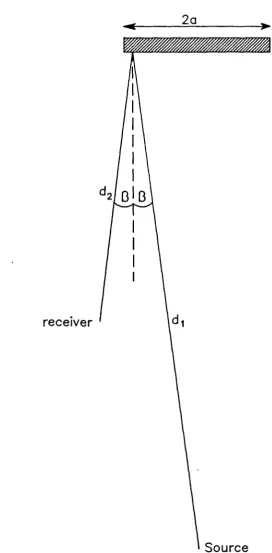
d1 Source distance to point of reflection (Figure 4.15) d2 Receiver distance to point of reflection (Figure 4.15)
Maximum depth of quadratic residue diffuser d. Characteristic distance
Deutlichkeit
E(t) Exponential energy decay
E0(t) Initial energy of exponential decay EDT Early decay time
ELEF Early lateral energy fraction Frequency
FT Fourier transform
Green's function Half panel height
h(t) Impulse response of panel
H(o) Measured transfer function for two microphone measurement
H2(co) Measured transfer function for single microphone measurement
H(o) Transfer function between two microphones i-1
IACC Inter aural cross correlation coefficient (i) Wavenumber
1
MOD
nmax
lit
p(t) or p(f) Po P8(t) Pi(t) PAO) P1/2(f,0) P't(fr) P'1/20,01 Pi(t) Pa pr(t) Pa(f) Q((A))
Q'xy2 or q(4)) Qxyi or Qi(w)
Half the largest panel dimension Sound pressure level
Fixed sound pressure level, taken to be 70 dBA Air absorption coefficient
Modulus
(i) Quadratic residue sequence number sequence (ii) Number of averages
Maximum number in quadratic residue sequence Prime number for generation of QRD
Integration limit for discretized impulse response
Unit vector at receiver in the direction of r (Figure 3.1) Normal to surface, pointing away from surface (Figure 3.1) 'Pressure
'Magnitude of point source
'Pressure measured using figure of eight microphone 'Incident pressure
'Full length diffuser pressure prediction 'Half length diffuser pressure prediction
'Full length plane panel pressure prediction for infinitely wide panel
'Half length plane panel pressure prediction for infinitely wide
panel
'Pressure at left ear
1Discretized impulse response components 'Pressure at right ear
'Scattered pressure 'Total pressure
Imaginary part of cross spectrum
Imaginary part of processed cross spectrum
Imaginary part of cross spectrum for measurement with the diffuser
Qxy2 or Q2(CO) Imaginary part of cross spectrum for measurement without the
diffuser
Vector from origin to receiver (Figures 3.1 and 3.3) _or Vector from origin to source (Figures 3.1 and 3.3)
Vector from a point on the surface to receiver (Figure 3.1) Vector from origin to a point on the surface (Figure 3.1) (i) Reverberant to early energy ratio
(ii) Reflection factor
Rxy( Ø ) Cross correlation function
Processed cross correlation function Surface area of room
Surface of integration S(a) Sine part of Fresnel integral
SI Subjective degree of spatial impression
SINC(x) SIN(x)/x
S 1 or
S
1(co) Cross spectrum for the measurement with the diffuserS 2 or
S
2(w) Cross spectrum for the measurement without the diffuser S' S'(G)) Processed cross spectrumS,a
(o)
Auto spectrum of loudspeaker microphone signal for measurement without diffuser presentSyy(w) Auto spectrum of diffuser microphone signal Time
Time interval for correlation integrals
T time
Centre time Room volume Well width
x coordinate of receiver (Figure 3.3) x(t) Loudspeaker microphone signal y(t) Diffuser microphone signal
B (i) Admittance
(ii) Angle of incidence and reflection (Figure 4.15) B. Variable used in Fresnel solution (Equation 3.18) Y Variable used in Fresnel solution (Equation 3.17)
Y2 Coherence function
c Variable used in formulation of Helmholtz-Kirchhoff integral equation (Equation 3.1)
13 (i) Angle of reflection (Figures 3.1 and 3.3)
(ii) Angle of incidence relative to an axis drawn through the ears of the listener
1 Wavelength
1 Maximum wavelength for which QRD produces 'optimum' diffusion
A min Minimum wavelength for which QRD produces 'optimum'
diffusion
0
il Auto correlation coefficient for left earth. Cross correlation coefficient between left and right ear 0 n. Auto correlation coefficient for right ear
a2 Variance
a
± a,z Variables used in Fresnel integrals (Equations 3.19 and 3.20) Time dependant velocity potential.r Time delay
Time delay between loudspeaker and diffuser microphones r .
r r Time delay between diffuser microphone and panel r a Time delay between loudspeaker microphone and panel
Time delay between loudspeaker microphone and diffuser
r r
microphone involving reflection off the panel (Figure 2.5) To Time delay between loudspeaker and loudspeaker microphone
ca Angular frequency
V Velocity potential
Chapter 1
Introduction
1.1 Introduction
Auditorium acoustics is a combination of objective and subjective effects. Even if the sound field within an auditorium is well defined, this still has to be related to the perception of the listeners. Modern auditorium acoustics is based on objective parameters. There are many such parameters [Cremer 1982, Kuttruff 1991a], an example is early lateral energy fraction. These parameters are known to be related to certain preferred subjective responses. By 'optimizing' the objective parameters, the preference of the audience will also be 'optimized'. For the example of early lateral energy fraction, the subjective feeling is one of being enveloped in a broad sound field; the jargon for this is spatial impression [Barron 1974].
This research project has investigated both objective and subjective effects. In particular, it has assessed the performance of finite sized surfaces such as reflectors and diffusers. The project has involved:
2. Development of methods to predict the scattering from finite sized surfaces.
3. Subject tests to find out how small a change can be perceived in the early sound field. The early sound field is the part of the impulse response most influenced by reflectors and diffusers.
1.2 Objective Measurements
The sound field within an auditorium can be defined by it's pressure impulse response. When designing an auditorium, an acoustician has two main methods for predicting such an impulse response: either physical scale modelling or computer modelling. Physical scale modelling is a well known and long established technique in room acoustics [Barron 1983b, 1987]. An accurate scale model of the auditorium is built, nowadays 1:50 scale is usually used. Then by working with frequencies 50 times the audible range, the performance of the auditorium can be judged. The models allow the acoustician to get a reasonable idea of how the auditorium will perform before the hall is built, so avoiding expensive mistakes in the real hall. Unfortunately, building models is time consuming and expensive. So in recent years there has been much interest in computer modelling.
3 method, and the ray tracing method; details of both methods can be found in Kuttruff [1991a Pages 282-287] or Stephenson [1990]. It is only in recent years, however, that there has been sufficient computing power to allow these methods to evaluate auditoria on desktop computers. Now many acoustic consultancies use computer modelling. Unfortunately, present day computer models have a major flaw, they can not properly predict the scattering from finite sized surfaces. One objective of this project was to improve understanding of these scattering processes. This was done through our theoretical predictions and measurements of the scattering from diffusing and reflecting surfaces. This will help scattering to be incorporated into computer models. An example of how predictions or measurements of the scattering from finite sized surfaces, can be incorporated into ray tracing models, is given in the next paragraph.
A ray tracing model literally traces rays around the auditorium, bouncing them off surfaces using Snell's law - i.e. angle of incidence equals angle of reflection. The sound rays are attenuated after each reflection according to the absorption coefficient of the surface. A popular approach to model scattering is to introduce a probability distribution function for the scattering direction after the ray reflects from the surface [Kuttruff 1991b]. To do this, the scattering properties of the surface needs to be known. It must either be measured or theoretically predicted.
method which used a pseudo-random white noise source signal was also very fast. Details of the measurement methods can be found in Chapter 2, along with a brief review of other possible systems.
A range of prediction methods have been tested, from the simple and fast, to the more rigorous and slow. For all surfaces tested, accurate prediction methods were found. As the more rigorous methods take a long time to compute, they may not be of practical use to acousticians and may be too slow for incorporation into ray tracing models. Consequently simple prediction methods were also looked at. These might have taken a matter of minutes or seconds to compute, where the more rigorous methods might have taken hours. With the more approximate methods, their limitations have been defined, in terms of the frequency ranges and receiver positions over which they work, and also the accuracy achieved.
5 Chapter 3 gives details of the theoretical prediction methods used. In Chapters 4 to 6 details of the comparisons between theoretical predictions and measurements for the scattering from the surfaces are given. Here the success, or otherwise, of each theory is considered.
Predicting the performance of diffusers is not just important to allow more accurate predictions of the sound field through computer modelling. Good concert hall design requires knowledge of the scattering performance of diffusers. Of the three types of panels tested, the most interesting were the quadratic residue diffusers (QRDs). A QRD consists of a series of wells of equal width but different depth, and was designed by Schroeder to give uniform scattering [Schroeder 1979]. Photographs of the QRDs used in a recently built concert hall can be seen in Plates 1.1 and 1.2. There have been comparatively few measurements to test the actual performance of QRDs [D'Antonio 1985, Strube
Plate 1.1 Quadratic residue diffusers in situ in a recently built concert hall. Plate 1.2 End view of a quadratic residue diffuser used in a recently built
9
1.3 Subjective Measurements
Although most of the current objective parameters which can be used to characterize a concert hall have been known for many decades, their use is not that widespread. The only exception is reverberation time, where measurement is simple and standardized. There are a number of different reasons for the objective parameters not being used: (i) there are many different parameters, many duplicating the same subjective effect; (ii) the measurements need equipment different from standard reverberation time measurements; and (iii) a consensus is only slowly emerging from the scientific literature. All these factors have resulted in a certain inertia in acousticians using the objective parameters. Their use, however, may well become more widespread with the increase in the use of computer modelling. Most computer models automatically produce a full range of the objective parameters.
changes to the early sound field. The first few reflections arriving at the listeners can be greatly influenced by the position, orientation and type of diffuser. This lead us to measure difference limen for early lateral energy fraction, inter aural cross correlation, centre time and clarity index. The results of these measurements are given in Chapters 9 and 10. The tests were done using an artificial sound field created in an anechoic chamber. The simulation system sounded natural subjectively. Also the key objective parameters - reverberation time, early decay time, clarity index, early lateral energy fraction and overall A-weighted sound pressure level - were all reasonable values when compared to values measured in real halls and preferred values measured in other subjective measurements. A description of the simulation system can be found in Chapter 8 along with details of the test method.
The results for the difference limens can be used in many ways: (i) they give guide lines as to how accurately the objective parameters should be measured; (ii) they stipulate to what accuracy computer models need to be able to predict the objective parameters; and (iii) they also tell acousticians whether changes to the positions and orientations of reflectors and diffusers will actually be heard by the audience.
11 many different surfaces, that the influence of diffuse reflections will be masked. In the early sound field, however, much fewer reflections arrive, and so listeners might be able to perceive a difference when the reflections are made more diffuse. Our interest was raised by Le Quartz in Brest, France. This is a theatre where the side walls have been lined with quadratic residue diffusers. Details of the measurements can be fund in Chapter 11.
The final subjective tests concerned the initial time delay gap. This is the time difference between the arrival of the direct sound and the first reflection. The initial time delay gap has been used by some as an objective parameters
The Measurement of Scattering from Finite
Sized Surfaces
2.1 Introduction
Before constructing a system to measure the scattering from surfaces, a survey of possible methods was done. This chapter begins with a brief overview of the methods available, including a discussion of their various merits. It was decided to develop a new measurement system based on the cross correlation function. Originally a two microphone method was used with white noise as a source. Unfortunately, although this method was accurate it was slow. Consequently, this was later superseded by a system using a pseudo-random white noise source, providing both fast and accurate measurements. This chapter gives full descriptions of the two methods. They had much in common, and are presented in historical order.
2.2 Possible Methods to Measure Sound Scattering.
13 field were required. If just the total field was needed, a simple single microphone measurement would have sufficed.
There are a number of methods available to measure the scattering from finite sized surfaces of the dimensions of surfaces typically found in auditoria. The main options are:
1. Directional microphone method. 2. Impulse source method.
3. Time delay spectroscopy. 4. Doublet source method.
5. Two microphone cross correlation method using a white noise source. 6. One microphone cross correlation method using a pseudo-random white
noise source.
2.2.1 Directional microphone method
normal to the panel (0 = 0°, 0 being the receiver angle), but as the scattering angle increases (0-n90°) the results will get more and more inaccurate as more and more of the direct sound is picked up by the microphone. Another criticism is that the method prevents the extraction of the total sound field, this would have to be measured separately.
2.2.2 Impulse source system
Using an impulse source is a common technique in acoustics [Barron 1984, Aoshima 1981, Ortega 1991]. For our measurements, once the time signal is captured the impulse response would be similar to Figure 2.1, consisting of an incident sound peak and reflected sound peak separated in time. (The impulse response in Figure 2.1 was measured by the single microphone cross correlation technique. Details of that measurement system is given in Section 2.4). Separation of the reflected sound and incident sound is then possible by consideration of arrival times. So it is simple to obtain both the scattered and
total field from the results. The main problems for an impulse measurement is that loudspeakers can not produce sharp impulses with high power. This results
in low levels at the microphone, and decreased signal to noise ratio. There are several solutions to this problem:
-_,
_
_I
15
-o ro
o
o 1-.
-1 1 1 1 1 I 1 1 1 1 0
N , 0 , N r0 "1- in (0 h
0 0 0 0
6000000
IIIIII1
(ii) Use half a period of a sinusoidal wave as a source. This allows more power to be fed into the loudspeaker and so reduces the number of averages [Barron 1984]. Unfortunately, the frequency response of the impulse created by part of a sinusoid is band limited, and so measurements have to be done several times to cover the full bandwidth required.
(iii) Use computer generated impulses based on the inverse of the loudspeaker's response [Aoshima 1981]. This can be used to maximise power output while producing a sharp impulse response.
Even when using the last two techniques, averaging is needed, and the measurement technique is slow.
2.2.3 Time delay Spectroscopy
17 There is a problem in that the reaction of the panel to a swept signal is unknown. The source is not similar to a music source.
2.2.4 Doublet source method
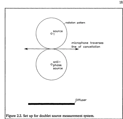
A Doublet source can be used to measure the scattering from surfaces [Dodd 1988]. If two identical sources of opposite phase are set radiating, the well known doublet source radiation pattern is created. There exists a line of cancellation along which a microphone can be traversed. This is illustrated in Figure 2.2. Along this line of cancellation the microphone picks up none of the incident sound, and measures the reflected sound only.
The system is limited by how accurately the two opposite phase sources can be produced, and also how accurately the microphone is positioned relative to the sources. The largest disadvantage of the system is that it does not allow full radial plots to be done as the microphone is constrained to a straight line. With the size of =echoic chamber which was available, this would have severely restricted the range of scattering angles which could have been measured.
2.2.5 Cross correlation methods
source
1
01i ,
microphone traverses ...-- line of cancellation ..-
7.-,
\\ radiation pattern
.411(
i
I anti—
1
'I I
\
0 phase 1\
\
/
source
\
/
/
I
,
,„
... ,--- - -
,..-'
Diffuser
[image:33.595.80.514.71.489.2]/
Figure 2.2. Set up for doublet source measurement system.
by subtraction and time gating. Unfortunately, using a white noise source means . that the measurement is slow, but this can be overcome by using a
pseudo-random noise signal. More details of these systems are given in Sections 2.3 and 2.4.
2.2.6 Summary of methods available
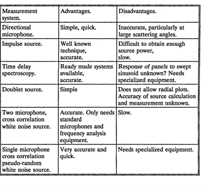
19 considered. The impulse source method, time delay spectroscopy and cross correlation techniques all provided possible ways to measure the scattering from the surfaces accurately. It was decided to develop the cross correlation technique, which to our knowledge had not been used before.
Table 2.1. Summary of possible methods for the measurement of scattering from diffusing and reflecting surfaces.
Measurement system.
Advantages. Disadvantages.
Directional microphone.
Simple, quick. Inaccurate, particularly at large scattering angles. Impulse source. Well known
technique, accurate.
Difficult to obtain enough source power,
slow. Time delay
spectroscopy.
Ready made systems
available, accurate,
Response of panels to swept sinusoid unknown? Needs specialized equipment. Doublet source. Simple Does not allow radial plots.
Accuracy of source calculation and measurement unknown. Two microphone,
cross correlation white noise source.
Accurate. Only needs standard microphones and frequency analysis equipment. Slow. Single microphone cross correlation pseudo-random white noise source.
Very accurate and quick.
.
Needs specialized equipment.
2.3 The Two Microphone, White Noise Source, Cross Correlation System
2.3.1 General principle of measurement system
The experimental set up for the two microphone cross correlation system is shown in Figure 2.3. A loudspeaker radiated white noise from one end of the anechoic chamber, the reflecting panel was placed at the opposite end. The pressure was measured by two microphones. The loudspeaker microphone was not far from the loudspeaker. The diffuser microphone was nearer the diffuser, and was rotated to allow the scattering from the panel to be measured as a function of scattering angle.
A cross correlation was calculated between the two microphones using a dual channel FFT analyzer. The pressures at the two microphones will be represented by x(t) and y(t) for the loudspeaker and diffuser microphones respectively. Then the two sided cross correlation function, R„y(r), is given by [Bendat 1986 1980]:
T
li
R ( mc) = —[ 1 f x(t)y(t+t)dt] T-.. T_T
21
VVVVV
VVVVVVVV
VVVVV
VVVII
L-a) 0 a) a u) n o L_ a) ...y 0
DC 0 o a _c
-o u) a
-S' 2 s... 0 -1-, 0 0 4-(1) Ce
n. 2
1
___J 0
• — I
1.-C e •C e
.=
,,,,--o a
_I M
'5-'4 00
A' 4 ji E
Le C 0 1.7, 0 Ti) L. '6 0 u9 0 0 `. a) C o
L,...; ..c ..., r% cri Er 0 ,_ a) C o _c a 9_
*--CD•M
s.-0 . _ E o -4-* L -0 LI-Cr) C . EL 16 ‘,,
L-0- -I-8 ci, a) 4-J ,- L. 0 t -0
-a n I -1-, a) u)
O .0
t
I
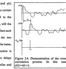
Figure 2.4. Demonstration of the cross correlation process. In this case y(t)=x(t-r ).
microphone signals x(t) and y(t) are compared, only when a certain time delay, r 1, is added to the microphone response x(t), will the two signals be identical. When such a time delay results in the two microphone signals being the same, the cross correlation function is large and finitel, at other delays the two signals are dissimilar and the cross correlation is zero.
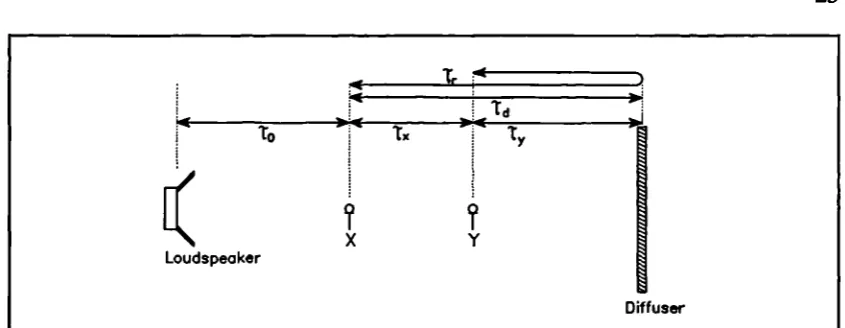
For the actual measurement with the diffuser, one such delay, r„ was equal to the time taken for the sound to travel direct from one microphone to another. Another delay, r, was the time taken for the sound to travel from one microphone to another reflecting off the panel. Figure 2.5 illustrates the 'definitions of these time delays. In this case the two microphone signals were not simply related by a time delay. However, the cross correlation function worked provided that the two signals are linearly related. So the various sound paths between the microphones had to be linear, including the reflection from the panel.
23
Tr 44
11( X
Loudspeaker
[image:38.595.85.508.81.245.2]Diffuser
Figure 2.5. Definitions of delays used in developing the theory of the cross correlation method.
An example of the measured cross correlation function is given in Figure 2.6. The incident sound and reflected sound can clearly be seen. There are two other 'secondary' peaks both at negative time delays (the second of the secondary peaks is to the left of the graph at too large a delay to be seen). The secondary peaks occur because the sound reflecting from the panel was picked up by the loudspeaker microphone. From the cross correlation definition, Equation 2.1, when there are two time delays at each microphone when the signals are similar, there are four correlation peaks. The secondary peaks are well separated in time from the incident and reflected sound, and so could easily be removed by time gating.
It can be seen from the cross correlation function, Figure 2.6, that the incident and reflected sound could be separated in the time domain. This process will be discussed in Section 2.3.3. A Fourier transform could then be taken of just the reflected sound to produce the processed cross spectrum. To remove the
4
o•_
-
%-Q.)
— _C
—I—, L.
— 03 0
4— C —
0 IP
- co oc n 4-_
>, —0
— 0 (I)
D
NO 03 —
I co
a)
- E
IIIIITII
CD N 00 d— 0
4- T-- CD 0
I 1111
d— N (\1
I
-4-a
I
24
2.2 is given by:
Si (w)
H(6)) -
xY//mac( GOSIPAO
25 loudspeaker microphone measured with no diffuser present. The difference in the responses of the microphones also had to be allowed for, this was represented by the transfer function between the two microphones, H(ø).
The resulting transfer function measured, H(w), represents the change in the sound wave of a continuous white noise source, travelling from the loudspeaker microphone to the diffuser microphone reflecting off the panel. This
where S/ (co) is the processed cross spectrum, S.(o) the auto spectrum of thexy loudspeaker microphone for the measurement without the panel present. A full derivation of Equation 2.2 is given in Section 2.3.2.
Analysis of the total sound field was identical except that the processed cross spectrum used in Equation 2.2 was calculated from the complete cross .correlation function minus the secondary reflections.
23.2 The theoretical basis for the cross correlation method
SO
y(t) = p(t—r) + f h(a)p(t-tr-a)da 2.3
where h(a) is the impulse response of the panel, and p(t) is the signal from the loudspeaker as it passes the loudspeaker microphone.
The loudspeaker microphone response is similarly:
CO
x(t) = p(t) + I h(a)p(t-2td-a)da 2.4
The instantaneous cross correlation between the two microphones is [x(t).y(0], and is given by:
-
-[p(t)+ f h(a)p(t-2cd-a)cla]ip(t-t) + f h(a)p(t-t r-a)da] 2.5
This can be expanded to:
.. [p(t)p(t-T)]
+[ f h(a)p(t)p(t-sr-a)cla]
+[ f h(a)p(t-ltd-a)p(t-Tx)da] 2.6
+[f h(a)p(t-2t d -a)da • fh(a)p(t-tr-a)da]
27 reflections - can now be eliminated. This leaves just the reflected sound. The instantaneous processed cross correlation product is then:
[x(t)7(t+t)]1 = f h(a)p(t)p(t-T Oda 2.7
An estimate of the full processed cross correlation, R( r ), is then derived from
Equation 2.7 by applying the cross correlation definition shown in Equation 2.1:
Rixy(T) = f [X(0)(t+T)]Idt 2.8
-T
Using Equations 2.7 and 2.8, and the fact that the auto correlation function is the cross correlation of a function with itself, it can be shown that:
R.,y1 (T) f h(a)R.(t 2.9
-T
Finally, taking the Fourier transform of Equation 2.9 and rearranging gives:
(4)) H(6.)) •Y
S(c)
with H(w) = F71h(a)]e-''
where SC(6)) is the processed cross spectrum; S.(w) is the auto spectrum of the loudspeaker microphone for the measurement without the diffuser; FT denotes a fourier transform; and H(6)) is the required transfer function. For the definition of the transfer function see discussions about Equation 2.2.
To get the full measurement Equation 2.2, an extra transfer function is included to allow for the different microphone responses. The effect is that the instantaneous cross correlation is in reality convolved with the transfer function between the two microphones. So in Equation 2.8 [x(t).y(t)]/ should be replaced by Hmiclx(t).y(t)r (* denotes a convolution). The microphone transfer function then appears on the denominator as a simple multiplier when the Fourier transform is taken. For further details on cross correlation measurement systems see Bendat and Piersol [Bendat 1980].
233 Separation of incident sound and reflected sound
For the scattered field to be found the direct sound had to be eliminated from the cross correlation. This was done by two process, subtraction and time gating. Figure 2.7 illustrates the processes. The tail of the incident sound peak overlaps with that of the reflected sound peak, this means simple time gating would not be sufficient. Consequently, the system was measured twice, once with
29
IIII
L() .4- ro (NI ,
0 0 0 0 0
0 tr) _c _C 4 a.) ED a) _C 4-* 0 0 4-0 (f) o 4-Tv o ci
I.-o
0 Cl) cn 0 L. C.) ca)cr)
6 cv
L-.
L_
01) (1) L_ 4.17. IIIIII o , 0 N 0 In 0 '4" 0 LO 0 CO 0
a)
_C
i
_0 4-•
ro L
o
4-C o :4-7, c.) C
-F 111
11') .4- rf) N
0 0 0
o di0
I 1 I I I I
, N rr) "I- LO CO
0 0
0 0 0 0I I I I I I
N
o I
o
30
C "
o
C.) 0 U) a) 747_ 0_
Q) (/)
c -o o
—(1) o
-o a —
a) E E
I 1:5 n 0 S
1 1 1 1 1 1 1 1 1 1
00 "I' o 00
o o o o
c3
0
31
2.3.4 Microphone calibration
A pair of matched Briiel and Kjmr microphones (4183) were used for the measurements. The use of matched microphones increases the coherence between the microphone signals and so improved the accuracy of the measurement. Despite the microphones being matched, the responses were slightly different and so a calibration was necessary. To do this the microphones were placed a few centimetres apart at one end of the anechoic chamber, equidistant from the loudspeaker, which was at the other end radiating white noise. The Ono Sokki dual channel FFT analyzer then allowed the transfer function to be directly measured via the standard cross spectrum method [Bendat
1986 1980].
23.5 Movement of the diffuser microphone.
33
35
2.3.6 Assessment of measurement accuracy
Many measurements using white noise use the coherence function as a test for accuracy. The coherence function for two pressure signals x(t) and y(t) is defined as [Bendat 1986 1980]:
y .v2 (w) _ 1.546))1 2
S.(co)Syy(o))
where S„(0) is the cross spectrum of the two signals and S.(6)) and S(w) represent their respective auto spectra. It can be shown that 0 . y2 (c)) 5.. 1.
If x(t) and y(t) are related by a single linear transfer function h(t) so that y(t).----h(t)*x(t), then the coherence function is one (* denoting convolution). Imperfect systems such as those with an amount of coherent background noise in either of the signals, produce a coherence of less than 1. So the coherence gives a measure of how much noise there is in a system.
Unfortunately, in our system the coherence function was complicated by the presence of more than one main correlation peak. This lead to the coherence function having a comb filter type response. An example is shown in Figure 2.8. This was exacerbated by the presence of the secondary reflections. These reduce the coherence, yet do not decrease the accuracy of the measurement as they were easily eliminated by time gating. Consequently, the coherence function was not a good measure for testing the accuracy of this system. Therefore direct evaluation of the variance of the system was used.
s....0...nnnnn
C--...
_
_
X
Y
0
I I I I I i i
1.-7 01 1.1.
0
-v.-
37 White noise is a random signal, and so it requires averaging to get an accurate estimate of functions such as the cross correlation function. It was necessary to assess how many averages would be needed to get a certain accuracy. The error formula was derived by combining the error formulations for cross spectra and auto spectra given in Bendat and Piersol [Bendat 1980]. The derivation can be found in Appendix 1. It shows that the variance of the resulting transfer function is:
a2lHool - [ 1SCy(o))12
]i 02
1 Sixy0.10 ) I + G215=001114,(0 )1 2 1 .5.(6))1 2 1 .514 6))1 2 IS.0012
2.12 where a2 denotes variance; S.; (G) the processed cross spectrum; S.(6)) the auto spectrum of the loudspeaker microphone for the without diffuser measurement;
and 1-1.,k(G)) the transfer function between the two the microphones.
The derivation assumed that:
. 1. The signals were noise free. Reasonable in laboratory conditions.
2. The error in the microphone calibration was small. As the microphones are very close together in the calibration, the coherence between them was one. As the calibration was only done once in each session, it could be done with a very large number of averages to eliminate random errors. Both these conditions made the error assumption reasonable.
loudspeaker microphone signal with no diffuser present. This assumption was tested as detailed in the following paragraphs.
The theoretical error formula was tested against measurement. To do this twenty identical measurements of the transfer function of a simple plane panel were made and the random error calculated. Standard statistical formulations were used [Bendat 1980]. In Figure 2.9 the experimentally derived percentage random error and theoretically expected values are shown for 128 averages. It can be seen that there was good agreement between the experimental and theoretical random errors in the locations of the minima and maxima. In general the theoretically predicted variance was greater than the experiment, due to the fact that the processed cross spectrum and auto spectrum for the measurement without the diffuser were not truly independent. This lead to some errors being counted more than once. So assumption 3 above was good except that it lead to an over estimation of roughly 2% in the random error.
0
2II
n•••n•-n
n•1010
•
n••••nnnn•••••.--.
I I I I 1 I I I I I I
.4- N 0 03 CO •cl- N 0 CO CO NI- N N N N
=
•
nnnnn/10
••n•n•_•••n
-•••
.11•• .1M•
39
microphone, a reduction in the signal to noise ratio, and consequently a reduction in accuracy.
For the experiments, 1024 averages were used to get an average 3.5% accuracy for the transfer function. The formulation 2.12 above, allows the calculation of the errors for other number of averages. The error value of 3.5% is for the random error and does not include bias errors. Bias errors could have been caused by such effects as: unwanted reflections off equipment; bad construction of the panels; and misalignment of equipment.
2.3.7 The problem with using white noise
Unfortunately, there was a major drawback in using white noise as a source, the averaging required to obtain a reasonable estimate of the transfer function was very time consuming. To measure the scattering from a single panel to a 3.5% accuracy required 1024 averages for each receiver position and took 24 hours. Consequently, a much faster maximum length sequence, pseudo-random noise source measurement system was used instead.
2.4 One Microphone, Pseudo-Random Noise Source, Cross Correlation Method
-o
-o n c
cn
a E
t
- -
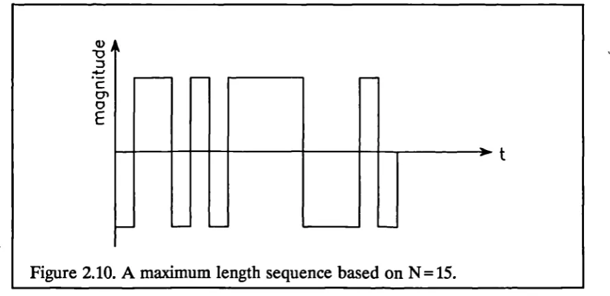
-Figure 2.10. A maximum length sequence based on N=15.
41 sequence is a set of pulses of different widths but equal magnitudes, the width of the pulses are determined by the maximum length number sequence [Rife 1989, Herbert 1983]. An example is shown in Figure 2.10 for a short sequence based on N=15. Over the length of the signal the order of the impulses is unique, so in a similar way to white noise, cross correlations and similar functions can be calculated. Yet the maximum length sequence is a deterministic signal, which means that for relatively noise free microphone signals, only a single cross correlation measurement is needed. So the time consuming averaging process used with a white noise source is no longer needed. Accurate
measurements of cross correlations can be obtained in seconds, where using white noise would take minutes.
[image:56.595.85.530.370.586.2]that a simple cross spectrum calculated in the anechoic chamber was accurate to .02% with no averages.
The actual technique for measurement was nearly identical to the two microphone cross correlation method. The major difference was that the reference against which the cross correlation was calculated was no longer the loudspeaker microphone but the maximum length sequence source signal generated by the computerized measurement system. This provided a noise free input source for the cross correlation function, which was necessary to exploit the deterministic nature of the pseudo-random sequence. This meant that there was no need for a relative calibration of the microphone pair. A calibration was still needed of the responses of the loudspeaker and other equipment. The new experimental set up is shown in Figure 2.11.
a) c o _c a-0
<
43 -fVVVVVVVVVVVVVVVVVVVVVV
L_ L-CD 0 _Y a 4-, 0 a) a.) a. Cl) -0 D 4-a) ct 0 .0 0 •-, L_ a) _o0 L.C E
_J 4((‘ (C.' 3 I- a _c c) 0 o _c 0 a) c c 1-c 52 o .4= o m
1\AAAAA/\AAAAAAAAAJV\AA
AA
L-a) L_ 4= q) 1= o ECL <
Crl C
0_4_, 61) 0
ri; 1-1:0 . a
C 0-. . - -3 o _0
0
t -0L..
0 0
0
L_
0-4a) ../ -4.
_.,-0 Z (1)
a_ a_ v)
EE ___, M
0
2.13
H2(co) - syyoz)
where S „y(w) is the processed cross spectrum, and S(w) the auto spectrum of the microphone signal with no diffuser present. A similar analysis to that given in Section 2.3.2 can be used to derive this formulation.
A commercial implementation of the maximum length sequence technique on a portable personal computer was used. This was the MISSA package. All other equipment, like the microphone control system were the same as for the two microphone method. The need to control the microphone position from the computer, meant the author had to develop customized computer programs using the device drivers provided, to supplement the measurement system.
2.5 Reasons for Measuring the Scattered and Total Field.
When measuring the performance of diffusers at low frequency both the scattered and total sound fields were checked against theoretical predictions. In the actual auditorium it is only the total field that is heard by the audience, and so interest in the scattered field could be questioned. However, there were several reasons for needing to look at the scattered field:
(i) At low frequency the total field was a simple picture, having a few minima and maxima which are well separated. This made comparison between theory and experiment easy. At high frequency, however, the interference pattern in the
45 total field became extremely complicated and vast varying. A small change in receiver or panel position resulted in a large change in the measured field. It was no longer simple to compare total fields, and so the scattered fields had to be used.
(ii) The performance of the quadratic residue diffuser is defined in the scattered field. It is claimed that it produces 'optimum' diffusion - i.e. uniform scattering of sound to all angles. This could only be tested in the scattered field.
(iii) When the results of scattering measurements are incorporated into ray tracing models, a simple probability distribution of the ray angle at each reflection is used [Kuttruff 1991b]. This distribution is determined from the scattered field.
2.6 Displaying of Results
2.7. Conclusions
Chapter 3
The Theoretical Prediction of Scattering from
Reflectors and Diffusers
3.1 Introduction
Many wave phenomena have been solved via the Helmholtz-Kirchhoff integral equation, whether these be electromagnetic or acoustic waves, radiation
or scattering. This investigation have concentrated on the application of various solutions of the integral equation to predict the scattering from reflectors and diffusers commonly found in auditoria. The prediction methods had varying degrees of simplicity, computation time and accuracy.
3.2 The Helmholtz-Kirchhoff Integral Equation
3.2.1 Definition of the Helmholtz-Kirchhoff Integral Equation
e G(rE)
-Ir-E,1
3.2 project the constant frequency form of the theorem was used. This gives the pressure p(x) for one point source as [Pierce 1981 pages 180-182]:
p(r) = 4
e
3.1
dS
3.1 + PA-Ed
where pi(1-4) is the sound pressure direct from the source; G(L-1 6) the appropriate free field Green's function; and the unit vector normal to the surface, pointing out of the surface. E can have values of 0,1/2 or 1 depending
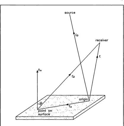
respectively on whether the point r lies within the reflecting object, on the surface of the reflecting object, or external to the reflecting object. Figure 3.1 shows the definition of the vectors used.
The derivation of Equation 3.1 is a well known problem and can be found in many standard texts [Pierce 1981 pages 182-, Ghatak 1979, Burton 1973], and so shall not be discussed here. Only the application of the equation will be discussed.
49
Figure 3.1. Definitions of vectors used in theoretical prediction methods.
origin
3.2.2 Local reacting admittance assumption
Helmholtz-Kirchhoff integral equation, Equation 3.1, the term in GvP.n., vanishes for a rigid surface as the velocity normal to the surface is zero. Consequently, there are no problems in defining an exact admittance which is also zero.
For surfaces with non zero admittance, the assumption of the local reaction needs to be justified. In most of the theoretical prediction methods used in this work, the complex shape of the quadratic residue diffuser (QRD) was approximately represented by a simple box with a variable admittance on the surface. Consequently, tests were necessary to examine the validity of the local reaction admittance assumption for the QRD. The representation of the QRD in the theoretical prediction methods is detailed in Chapter 6, along with the tests of the validity of the local reacting admittance assumption.
3.3 General solution method
51 the surface pressures and velocities. The problem is that the surface pressure and velocities depend not only on the sources, but also on the surface pressures and velocities themselves. In the past, approximations for the surface pressure were commonly used, one such example is the Kirchhoff approximation. In more recent decades the increase in computing power available has meant that a rigorous numerical solution taking into account of the mutual surface interactions is possible. These methods are outlined in more detail in Sections 3.4 to 3.6.
All surfaces tested allowed exploitation of symmetry to greatly reduce computation time. Symmetry was exploited in all the theoretical prediction methods.
3.4 3D Boundary Integral Method
This method is a rigorous numerical solution of the Helmholtz-Kirchhoff . integral equation, the values of the surfaces pressures being obtained via
Once the surface has been discretized, a set of simultaneous equations can be set up for the surface pressure using Equations 3.1 and 3.2, with r being taken as positions on the surface. Each equation gives the pressure on a particular surface element, as a sum of the contributions from the sources, and a sum of the contributions from all elements. The simultaneous equations are solved via the CHIEF method [Schenck 1968], giving values for the surface pressures on each of the elements.
If the set of simultaneous equations were solved alone, it would be possible to get non-unique solutions at certain frequencies. These equate to eigensolutions of the physical body dimensions. To obtain the correct unique solutions, the fact that the pressure is zero inside the surface is used as a constraint. Formulations of Equation 3.1 with r chosen at interior points are added to the matrix to form an over determined system. The number of interior points is increased until convergence of the solution is achieved [Schenck 1968]. In general one interior point was sufficient to ensure convergence of the surface pressures and velocities. However, it is possible that the single interior point could equate to a node of the eigensolution of the physical body dimensions, and so the interior point would still fail to ensure a unique solution. Therefore, using two interior points was preferred.
3.3
3.4 53 computer program implementation of the method was used in this work [Lam 1990].
3.5 Solution of the Helmholtz-Kirchhoff Integral Equation in the Thin Panel Limit.
Consider a rectangular panel represented in the 3D boundary integral method by a set of surface elements covering all sides of the body. When the panel becomes extremely thin, the 3D boundary integral method breaks down because there is a discontinuity in the pressure across the surface. Terai has given a solution for a perfectly rigid panel in the limit when the panel becomes infinitely thin [Terai 1980].
The derivation requires not only the Helmholtz-Kirchhoff integral equation given in Equation 3.1, but also the first order derivative form. Fork on the surface, Equation 3.1 and it's first order derivative are given by:
1
f jf a a
Iv = -27- j -G02-Q aTt p(t) 4-
p
(t) a---1--tG(E-E)dsit s . s
+ 2Pi(r -Ed
a2 0 _
aP - 1
ilf- a
G(r-r)
ap
(E) + P(L)cr(E-Es)ds ati , 27c s art , an s an an, s
api(E-r0)
+2
3.5
3.6 where lir is the normal to the surface at r.
Consider the situation when a rigid panel reduces in thickness to a infinitely thin body. This is illustrated in Figure 3.2. In that case if j is written as it can be shown that Equations 3.3 and 3.4 become:
a
pv ap(r.2)
P(
C
)+P(E2
)ff
{-c(r-t3)(a
ail )
.7c
s
fpv-Ars2AlGtr-ry ds
+ 2P1(r-to)
ap(c) ap(r2) _
S.
ail,.
1 ff{-G(E-01-fP(Ci)--Ars2)]
27t
5
an,
azt a2dS [PV -P(C2ManG(E-r)
OP,(t-rd
This method has been applied to rigid panels only, and so Equations 3.5 and 3.6 can be simplified further. The velocity terms of the two equations must be zero as the velocities must be equal and opposite on either side of the panel. This then leads to:
55
3.7
3.8
a
p(r)-T(L.2* ) = —1 HEX( )-p(r 2A—G(t-rs)dS
2 .7c 31 3 an
s
+ 2pi(E-Ed
o =
-
et-ff rp(r„)-pcz,2)] a.a2a.G(E-E)ds
s
,
+2
apAr-Edaar
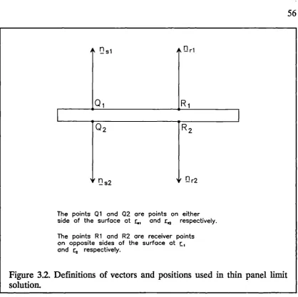
The solution method for the thin panel integral Equations 3.7 and 3.8 is similar to the 3D boundary integral method. Again the surface is discretized, but this time on one side only. So this method just over halves the number of elements needed to represent a thin panel when compared to the 3D boundary integral method. The surface pressures and velocities are again assumed constant across each element. A set of simultaneous equations are constructed and solved in terms of the pressure difference across the panel using Equation 3.8. Once the surface pressure differences are known a simple numerical integration of the following equation, derived from Equation 3.1, gives the external pressure:
P(E) =
Til-ffixt„)-xtam-l-G(t-Exs
n
S+ 4E-Ed
If the surface pressures are needed these can be obtained from the values for the surface pressure differences and from Equation 3.7.
A n s1 A[1- r1
Q2
V r-1 r2 v 0s2
The points Q1 and 02 are points on either side of the surface at r„, and r,,, respectively.
[image:71.595.89.508.62.479.2]The points R1 and R2 are receiver points on opposite sides of the surface at r , and [2 respectively.
Figure 3.2. Definitions of vectors and positions used in thin panel limit solution.
57
3.6 Transient Model
It is possible to use the full time dependant form of the Helmholtz-Kirchhoff integral equation, instead of the constant frequency version, to derive the surface pressures. This is given by [Kawai 1990]:
_ f ([41 a ( 1 ) [8413( 1 )ar-rs
4itei J
ail L —E C at E—r s anss s
-[-a-i—V](---)}dS +
irAt-tolt)
azt L—E
S s
where [4r] =
cit
s,t-(1-16)/c) and is the full time dependant form of the velocity potential, and c the speed of sound.To solve the time dependant form the surface is again discretized. It can be shown from the integral equation [Kawai 1990, Mitzner 1967, Friedman 1962] that the velocity potential and it's derivative on the surface can then be represented by the incident velocity potential from the source plus contributions from the other elements at previous times. This is an exact solution and not an iterative method. Problems arise because the convergence of the surface velocity potentials can be very slow. When choosing the elements it is necessary to satisfy the quarter wavelength condition so that the pressure variation is well represented. It is also necessary that any variation within any time step is restricted to one element. This leads to a very small time step, and hence slow convergence.
The method has advantages over the constant frequency methods in that once the impulse response has been calculated, the full frequency response can easily be obtained by a Fourier transform. However, the model needs further development, particularly for non-rigid bodies as the formulation of admittance in the time domain is unclear. Unfortunately, time did not allow development of the model in this project. It does offer an alternative solution method to the more standard constant frequency methods.
3.7 Kirchhoff Approximate Solution
59
P(E) = P i(r)(1 + R) 3.11
VP(4) . Us = -i0kP(E) 3.12
where B is the normalized locally reacting admittance; R the local reflection factor; Pi the incident sound pressure on the surface; and k the wavenumber. For plane wave reflections, these are related by:
p =(..--L4--?)co5(a) 3.13
(1+R)
where
a
is the angle of incidence.This approximation alone allows much faster predictions as it eliminates the need to solve the matrix of simultaneous equations for the surface pressures. A simple numerical integration of Equation 3.1, using the Green's function of Equation 3.2, and the boundary conditions of Equations 3.11 to 3.13, yields the external point pressure.
3.8 Fresnel and Fraunhofer Approximate Solutions
former method is a solution nearer the panel and requires the use of the standard Fresnel integrals.
The approximations involved for both solutions are similar, except that the Fraunhofer solution is more stringent about how close to the panel predictions can be done. For the Fraunhofer solution the receiver must be in the far field. The true far field pressure distribution is only achieved when the receiver distance is much larger than 1 and 1d 2, 1 being half the largest panel dimension [Pierce 1981 page 217, Kinsler 1982 pages 187-188]. The other approximations required for both prediction methods are:
(1) The source is many wavelengths from the panel ro»A. (2) The receiver is many wavelengths from the panel r»A.
(3) For a particular source and receiver position, over the range of the integration the angles subtended by the source and receiver to a normal to the panel do not vary significantly.
"(4) Over the range of the integration, the variation in the source to panel, and source to receiver distances are small.
61 To begin with, the Green's function and Kirchhoff's approximation for the surface pressure must be incorporated into the Helmholtz-Kirchhoff integral equation. This involves the combination of Equations 3.1, 3.2, 3.11, 3.12and 3.13 to produce the following expression:
ps(r)
=
ikil°
if [ e -
ist(r2 +rcl)
[(R(E)-1)+(l+R(E))COSOWS4n a r
2r0
The source is a point source of strength Po normal to the surface, and 0 is the receiver angle. For simplicity only the scattered field expression is shown. The incident sound field contribution seen in Equation 3.1 can be added in to Equation 3.14 to obtain the total field, if required. The analysis now differs
depending on the reflector being modelled.
3.8.1 Solution for rigid plane panels
For the rigid plane panel, R =1, the standard Fresnel-Kirchhoff diffraction formula results [Ghatak 1979]. From this the formulations for Fresnel and Fraunhofer diffraction can be derived. The derivations will not be repeated here. (Although as we are dealing with off-axis receivers as well as on-axis receivers, the solution slightly differs from the more usual form given in Ghatak. Another derivation of the Fresnel solution can be found in [Leizer 1966]). It can be shown that in the far field the Fraunhofer solution is a SINC function - i.e. SIN(x)/x. The Fresnel solution results in the Fresnel integrals, the numerical solutions of which can be found in standard texts [Abramowitz 1965 pages 295-].
Aror
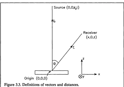
[image:77.595.90.507.91.382.2]Origin (0,0,0)
Figure 3.3. Definitions of vectors and distances.
3.15 Figure 3.3 shows the definitions of panel, receiver and source positions used in these two solutions. The panel front is taken to be on the
z =0 plane; the
source lies on the panel normal, drawn through the panel centre. The receiver and source are on the y=0 plane. In this case the Fraunhofer solution for the scattered pressure is-4thapoSINC( kx--a-)COS(0)e -Lk(r4)+6
r PA) =
where a and h are half the width and height of the panel; 0 the receiver angle; r and 1.0 the receiver and source distances to the centre of the panel; and x the displacement of the receiver in the x direction.