Swimmer selection optimization strategy research based on SPSS factor analysis

(1)

Journal of Chemical and Pharmaceutical Research, 2014, 6(3):1059-1068

Research Article

_{CODEN(USA) : JCPRC5}

ISSN : 0975-7384

Swimmer selection optimization strategy research based on SPSS

factor analysis

Mei Wei

1

and Keyi Jin

2

1

Shenyang Sport University, Shenyang, Liaoning, China

2

Institute of Physical Education, Dalian University, Dalian, Liaoning, China

_____________________________________________________________________________________________

ABSTRACT

Swimming is a sport that lays equal stress on endurance and technique, sound technique is guarantee of scientific exertion that makes contribution to swimming technique rationality and improvement direction. Utilize factor analysis method and integer programming model method; make application of mathematical model into competitive swimming. In research process, it respectively from athlete perspective adopts factor analysis method providing swimming strategy for athlete, from coach perspective utilize integer programming finding out optimal athletes assignment scheme and competition best total score; Make improvement based on precedence algorithm, apply sensitivity analysis, on the condition that optimal solution not changing, get athletes assignment performance intervals. Through this paper’s research methods, analysis routes and research results, it provides reasonable suggestions and theoretical basis for swimming technique.

Key words: Factor Analysis Method, integer programming, sensitivity analysis, swimming competition

_____________________________________________________________________________________________

INTRODUCTION

Swimming develops up to today, with every country swimming theories and technical research increasing improvement, training ways become more and more scientific, every country excellent swimmers’ competitive levels has been widely improved, competition victory or failure tend to be a moment affair [1]. Modern swimming has already become not just athlete physical ability, speed and technical competition; its competition result has slightly great correlations with competition strategy to great extent. So-called competition strategy, its essence belongs to mathematical planning problem. Apply modern mathematical research method into competitive sports, it starts since 1970s; American mathematician T.B.keller has established a mathematical model in 1973 for medium and long distance runners training that achieved remarkable results [1, 2]. Meanwhile, Ayers has combined mathematics, mechanics and computer with discus and improved throwing technique. Optimal control theory has been developing after Second World War; its basis is state-space concept. In 1960s, with digital computer technique and space technique rapidly development, driving by dynamic system optimization theory, optimal control theory starts to take shape as an important science branch [3-5]. Develop up to today; it has already achieved remarkable results in systematical engineering, space technique, economic management and other multiple fields. Optimal control theory is according to targets features, on the specified permissible control condition, let it operate as requests and make targets arrive at optimal value [6, 7]. Its mathematical essence is a functional extreme value problem, is a variation problem under a group of constraint conditions.

(2)

For competitive swimming, lots of problems have also been emerged that waited to be solved [8-10].

Factor analysis refers to statistical technique that research extracts common factors from clusters of variations. It was first put forward by British psychologist C.E. Spearman. Integer programming was formed into an independent branch after R.E. Gomory proposed cutting plane method; it has been developed into many methods to solve all kind of problems in 30 more years. With social science theory continuously development, current relative theories are in urgent need of blending in natural science, modern information technology. This research applies factor analysis method and integer programming model in researching competitive swimming problems with expectation of deep solving relative problems, especially in sports field.

SWIMMING PERFORMANCE INFLUENCE FACTORS FACTOR ANALYSIS MODEL Factor analysis method principle

Factor analysis is a way that tries to organize original multiple certain correlated indicators (such as

p

indicators) again into a group of new mutual independent comprehensive indicators to substitute original indicator. Common factors generate variance structure, and special factors explain every variable variance. The purpose is to make reasonable explanation as much as possible of original variables correlations and use it for simplifying variables dimensions and structure.

Factor analysis starting point is variable relative coefficient matrix, on the premise that less information loss, synthesize multiple variables (these variables are required to have strong correlations so as to ensure it can extract common factor from original variable) into a few comprehensive variables to research overall each aspect information multiple statistical method, and the few comprehensive variables represent information cannot overlap that variables are independent from each other, factor analysis dissolves original observation variables into common factor and special factor two parts. Factor model as following:

i M im i

i

a

F

a

F

a

F

X

=

₁ ₁

+

₂ ₂

+

....

+

ε

(

m

≤

p

)

₍₁₎

Among them i=1, 2, …, p, m that

X

=

AF

+

ε

F

1

,

F

2

,...

F

m_{is called common factor, is an unobservable}

variable,

A

=

( )

a

ij p×m is called factor loading matrix,

a

ij represents the

i

variable loading in the

j

factor,

i

ε

_{is special factor that is a part that cannot be included by previous}

m

_{pieces of common factors, and meet}

( )

F,

ε

=0

Cov _, F,

ε

_{are uncorrelated.}

Factor analysis is factor model focuses on a few unobservable potential variables (that is common factor) and

abandon special factor. If the first main common factor

F

1_{cannot represent original}

P

_{pieces of indicators}

information, then consider to select the second common factor

F

2_{that is to select the second linear combination. In}

order to effective reflect original information,

F

1_{known information is unnecessary to appear in}

F

2_{, by that}

analogy, it can construct the third, fourth... the

p

common factor. General steps of factor analysis:

(1) Similar to principal component analysis, calculate

x

k _and

s

k

(

k

,

j

=

1 ,

2 ....,

m

)

_{, establish basic equations.}

(2) Use principal component analysis method to determine factor matrix

A

.

(3) Varian orthogonal rotation, extreme variable coefficient (tend to 0 or 1 as much as possible) (4) Get factor score function, calculate sample factors scores.

Model establishment

(3)

[image:3.595.182.432.90.181.2]

Table 1: 2012 London Olympic Games every country athlete’s 1500 meter free stroke partial indicators data

\ 0-300 300-600 600-900 900-1200 1200-1500

China 172.63 175.52 176.17 176.32 170.38

Canada 174.12 176.72 177.7 177.69 173.4

Tunisia 175.61 177.85 177.32 177.07 172.46

South Korea 173.67 177.09 179.32 181.45 179.08

Italy 177.63 178.3 179.24 179.46 177.29

America 178.71 180.2 179.13 178.27 176.68

Poland 177.75 180.02 179.59 179.93 177.03

Britain 178.41 180.99 180.72 181.48 179.16

Factor analysis hypothesis: Each common factor is independent from each other, special factors are also independent from each other, common factors and special factors are independent from each other.

[image:3.595.194.418.299.349.2]

Apply SPSS software Linear process in carrying out factor analysis of data, firstly make KMO test and Bartlett test on data, carry out factor analysis of observation sample data whether suitable or not, and then further get correlated coefficient matrix as well as its feature values, contribution rations as well as accumulation contribution ratios and so on.

Table 2: KMO and Bartlett test a

Sampling sufficient degrees Kaiser-Meyer-Olkin measurement .705

Bartlett sphericity degree test

approximate to chi-square 49.359

df 10

Sig. .000

a. Based on correlation

From Table 2, it is known that KMO value＝0.705, Sig=0.00001. According to statistician professor Kaiser provided criterion, KMO＝0.705>0.5 is relative proper for factor analysis; Sig=0.00001<0.05 indicates that through Bartlett spheroid test prove that its correlation matrix is not a unit matrix, factor model is suitable.

Reuse SPSS software making factor analysis of data, get following results that all original variables general

statistical description (Table 3), including average number

x

i_{, standard deviation}

σ

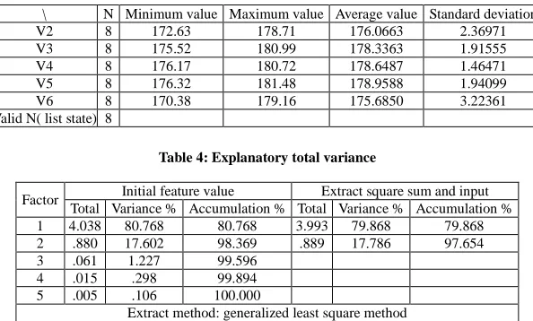
Xi_{and analytic case number,} explanatory total variance refers to Table 4.

Table 3: All original variables general statistical description information

\ N Minimum value Maximum value Average value Standard deviation

V2 8 172.63 178.71 176.0663 2.36971

V3 8 175.52 180.99 178.3363 1.91555

V4 8 176.17 180.72 178.6487 1.46471

V5 8 176.32 181.48 178.9588 1.94099

V6 8 170.38 179.16 175.6850 3.22361

[image:3.595.157.454.483.662.2]

Valid N( list state) 8

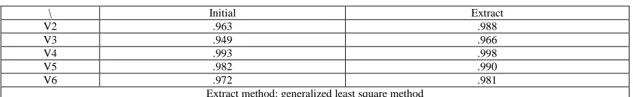
Table 4: Explanatory total variance

Factor Initial feature value Extract square sum and input

Total Variance % Accumulation % Total Variance % Accumulation %

1 4.038 80.768 80.768 3.993 79.868 79.868

2 .880 17.602 98.369 .889 17.786 97.654

3 .061 1.227 99.596

4 .015 .298 99.894

5 .005 .106 100.000

Extract method: generalized least square method

(4)

[image:4.595.202.409.107.289.2]

factors (Table 5).

Table 5: Correlation coefficient matrix table

\ V2 V3 V4 V5 V6

V2

Pearson correlation 1 .943** .741* .402 .590

Significance(two sides) .000 .036 .324 .123

N 8 8 8 8 8

V3

Pearson correlation .943** 1 .829* .550 .677

N 8 8 8 8 8

V4

Pearson correlation .741* .829* 1 .906** .961**

N 8 8 8 8 8

V5

Pearson correlation .402 .550 .906** 1 .951**

N 8 8 8 8 8

V6

Pearson correlation .590 .677 .961**.951** 1

N 8 8 8 8 8

**. It is significant correlated in .01 horizontal(two sides). *. It is significant correlated in 0.05 horizontal(two sides).

According to above data, draw out feature root screen plot figure (as Figure 1), combining feature root curve inflection point and feature root value.

Figure1: Feature root screen plot

From Figure1, it can get first feature value and second feature value have larger change range, and can consider to take previous two factors as common factors to carry out factor analysis.

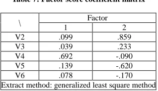
Common factor variance ratio (Table 6) evaluation indicator common degree is 0.85 bigger than all indicators that indicate model basically explains every evaluation indicator all variance and no need special factors.

Table 6: Common factor variancea

\ Initial Extract

V2 .963 .988

V3 .949 .966

V4 .993 .998

V5 .982 .990

V6 .972 .981

[image:4.595.80.534.681.751.2]

(5)

[image:5.595.227.386.112.204.2]

Factor score coefficient matrix (Table 7) that is factor analysis final result. Through the coefficient matrix, it can express common factors as each evaluation indicator linear combination.

Table 7: Factor score coefficient matrix

\ Factor

1 2

V2 .099 .859

V3 .039 .233

V4 .692 -.090

V5 .139 -.620

V6 .078 -.170

From that, it can get the first and second common factors expressions:

5 4

3 2

1

0 .

099 *

stdx

0 .

039 *

stdx

0 .

692 *

stdx

0 .

139 *

stdx

0 .

078 stdx

Z

=

+

₍₂₎

5 4

3 2

1

2

0 .

859 *

stdx

0 .

233 *

stdx

0 .

09 *

stdx

0 .

62 *

stdx

0 .

17 stdx

Z

=

+

−

₍₃₎

Total score function:

(

79 .

868 Z

₁

17 .

786 Z

₂

)

/

97 .

654 Z

=

+

₍₄₎

Among them,

stdx

i

(

i

=

1 ,

2 ,

3 ,

4 )

_{represents evaluation indicator variable after standardization:} )

4 , 3 , 2 , 1 ( / )

( − =

= x x i

stdx

i

x i i

i

σ

Total score function after simplifying:

1 2 3 4 5

0.2374 *

0.0743*

0.5496 *

0.0008*

0.0328

Z

=

stdx

+

stdx

+

stdx

+

stdx

+

stdx

(5)

Due to factor analysis model coefficient matrix reflects correlation extent between original variable and common factors, according to score expressions after simplifying, it can get that the first phase and the third phase have larger coefficients, therefore athlete in 0---300m, 600m---900m such two swimming journey, it cannot loosen and speed cannot too slow, especially in 600---900m such phase swimming journey, athlete speed should be fast, impulse in other phases’ swimming journey doesn’t need to be so fiercely so that can improve athlete swimming performance.

INTEGER PROGRAMMING MODEL Integer programming

0-1 programming is a kind of special pure integer programming. Solve 0-1 programming implicit enumeration method has no need to use simplex method solving linear programming problems. Its basic thoughts start from all variables equal to 0, successively appoint some variables into 1 till get a feasible solution and regard it as current best feasible solution. Hereafter, successively test variables equal to 0 or 1 combination so that let current best feasible solution get continuously improvement, finally get optimal solution. Implicit enumeration method is different from exhaustion method, it don’t need to enumerate all feasible variables combinations one by one. Through analysis, judging, it eliminates lots of variables combinations as optimal solution possibility. So they are implicit enumerated. Implicit enumeration method essence is also branch and bound method.

Model establishment

(6)

[image:6.595.160.457.89.141.2]

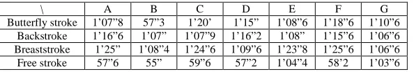
Table 8: 7 athletes’ four swimming postures 100 meter average performance

\ A B C D E F G

Butterfly stroke 1’07”8 57”3 1’20’ 1’15” 1’08”6 1’18”6 1’10”6

Backstroke 1’16”6 1’07” 1’07”9 1’16”2 1’08” 1’15”6 1’06”6

Breaststroke 1’25” 1’08”4 1’24”6 1’09”6 1’23”8 1’25”6 1’06”6

Free stroke 57”6 55” 59”6 57”2 1’04”4 58’2 1’03”6

Record A, B, C, D, E, F, G respectively as i=1,2,3,4,5,6,7;Record butterfly stroke, backstroke, breaststroke, free stroke respectively as swimming postures, record athlete

i

the

j

swimming posture 100meter best performance

as

c

ij

( )

s

, then Table 8 can express as Table 9.

Table 9: 7 athletes’ four swimming postures 100 meter average performance

ij

c

_i

=

₁

_i=₂

_i

=

₃

_i

=

₄

_i

=

₅

_i

=

₆

_i

=

₇

1

=

j 67.8 57.3 80 75 68.6 78.6 70.6

2

=

j 76.6 67 67.9 76.2 68 75.6 66.6

3

=

j 85 68.4 84.6 69.6 83.8 85.6 66.6

4

=

j 57.6 55 59.6 57.2 64.4 58.2 63.6

Bring into 0-1variable

x

ij, if select athlete

i

to participant swimming posture

j

competition, recordxij =1_{, or else} record

x

ij

=

0

.

As following: 

 

=

gposture m

tselectswi esn

athleteido

gposture lectsswim

athleteise xij

min '

, 0

min ,

1

.

With requests of organizing into relay team,

x

ijshould meet below conditions:

Every athlete can only be selected one of four swimming postures (2) Every swimming posture can only have one athlete be selected.

Then it has:

(

)

∑

=

≤

4

1

7 ,...

2 ,

1

j

ij

i

x

(

)

∑

=

7

1

4 ,...

2 ,

1

i

ij

j

x

Therefore, when athlete

i

is selected with swimming posture

j

, use

c

ij

x

ij showing its performance, relay team total performance can be expressed as :

∑∑

= =

=

• =

4

1 7

1

)

7 ,...

2 ,

1 ,

4 ,...

2 ,

1 (

j i

ij

x

i

j

c

z

To sum up, swimming team’s relay team athlete’s selection problem 0-1 programming model can be described as:

∑∑

= =

=

• =

4

1 7

1

)

7 ,...

2 ,

1 ,

4 ,...

2 ,

1 (

j i

ij

x

i

j

(7)

(

)

(

)

{ }











=

≤

∑

= =

1 ,

0

4 ,...

2 ,

1

7 ,...

2 ,

1

1 .

.

7 1 4 1 ij i ij j ij

x

j

x

i

x

t

s

Establish target function as following:

74 73 72 71 64 63 62 61 54 53 52 51 44 43 42 41 34 33 32 31 24 23 22 21 14 13 12 11 6 . 63 6 . 66 6 . 66 6 . 70 2 . 58 6 . 85 6 . 75 6 . 78 4 . 64 8 . 83 68 6 . 68 2 . 57 6 . 69 2 . 76 75 6 . 59 6 . 84 9 . 67 80 55 4 . 68 67 3 . 57 6 . 57 85 6 . 76 8 . 67 min x x x x x x x x x x x x x x x x x x x x x x x x x x x x z + + + + + + + + + + + + + + + + + + + + + + + + + + + =











=

+

=

+

=

+

=

+

≤

+

≤

+

≤

+

≤

+

≤

+

≤

+

≤

+

)

4 ,

3 ,

2 ,

1 .

7 ,

6 ,

5 ,

4 ,

3 ,

2 ,

1 (

1

0

1

47 46 45 44 43 42 41 37 36 35 34 33 32 31 27 26 25 24 23 22 21 17 16 15 14 13 12 11 74 73 72 71 64 63 62 61 54 53 52 51 44 43 42 41 34 33 32 31 24 23 22 21 14 13 12 11

j

i

or

x

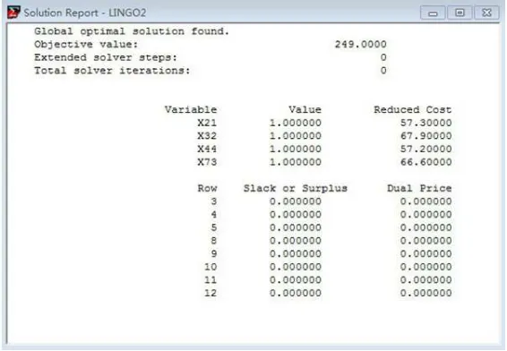
ij

[image:7.595.165.448.500.696.2]

Use LINGO program solving results as below Figure 2:

Figure 2: LINGO solution results

Apply LINGO software in calculating, it can get

x

21

=

x

32

=

x

44

=

x

73

=

1

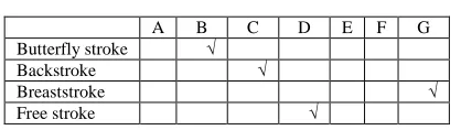
_{, therefore, selected athletes and corresponding}

(8)

[image:8.595.203.412.83.142.2]

Table 10: Selection scheme

A B C D E F G

Butterfly stroke √

Backstroke √

Breaststroke √

Free stroke √

That is a competition scheme that selects athlete B to take butterfly stroke→athlete C to take backstroke→athlete D to take breaststroke→athlete A to take free stroke. At that time, competition best total score is z=249s.

SENSITIVITY ANALYSIS Value coefficient

c

change analysis.

(1)

c

r_{is non basic variable}

x

r_coefficient

Now

c

r_{change only would influence on} N

c

N

c

B

N

1

−

=

σ

x

r_{check number, under requests to maintain}

optimal value, then it only needs to

0

1

=

+

∆

−

=

+

∆

≤

−

′

=

′

− −

r r r B r r r B r

r

c

B

P

c

B

P

σ

c

σ

That is when

∆

c

r

≤

−

σ

r_{, it can maintain optimal basis without changing.}

(2)

c

r_{is basic variable}

x

r_coefficient

Now due to

c

B_{changes, all non basic variables check numbers would change, under requests to maintain optimal}

value, then it needs to meet

0

1

≤

′

−

=

′

−

j B j

j

c

B

P

σ

_.

Here record vector

∆

c

B

=

(

0 ,

L

,

∆

c

r

,

0 ,

L

,

0 )

_{, then it has}

c

′

B

=

c

B

+

∆

c

B_.

From j

c

j

c

B

P

j

c

j

c

B

c

B

P

j

1

₍

₎

−

₌

₋

₊

_∆

′

−

=

′

σ

=

−

−1

−

∆

−1

=

−

∆

−1

≤

0

j B j j B j B

j

c

B

P

c

B

P

c

B

P

c

σ

It gets

(

,

x

var

)

1

iable

isnonbasic

and

j

P

B

c

_B _j

≥

_j

∀

_j

∆

−

_σ

.

From that, it can get optimum basis unchangeable

∆

c

r_{value range.}

Record

(

)

1

ij

a

A

B

−

=

′

, record basic variable

x

r _{code in base as}

s

_{, then}

∆

c

B

P

j

=

∆

c

r

a

sj

′

−1

, and

from

∆

c

B

P

j

=

∆

c

r

a

sj

′

≥

σ

j

−1

, it can get.

If

a

′

sj

>

0

_then

∆

c

r

≥

σ

j

/

a

′

sj

；If

0 <

′

sj

a

then

∆

c

r

≤

σ

j

/

a

sj

′

；If

0 =

′

sj

a

then obviously

∆

c

r

a

sj

′

≥

σ

j_{is true}

；

So that it gets optimal basis unchangeable

∆

c

r_{value range as:}maxj

{

σ

j/a′sj|asj′ >0

}

≤∆cr≤minj

{

σ

j/asj′|a′sj<0

}

If value coefficient

c

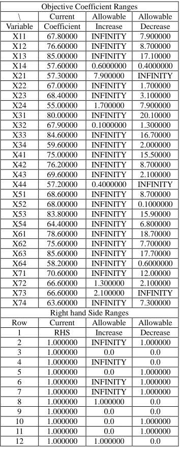
changes, then it not meet optimal condition any more (appear positive check number), then it needs to continue to make iteration solution by simplex method.

(9)

[image:9.595.218.395.89.531.2]

Table 11: Sensitivity analysis

Objective Coefficient Ranges

\ Current Allowable Allowable

Variable Coefficient Increase Decrease

X11 67.80000 INFINITY 7.900000

X12 76.60000 INFINITY 8.700000

X13 85.00000 INFINITY 17.10000

X14 57.60000 0.6000000 0.4000000

X21 57.30000 7.900000 INFINITY

X22 67.00000 INFINITY 1.700000

X23 68.40000 INFINITY 3.100000

X24 55.00000 1.700000 7.900000

X31 80.00000 INFINITY 20.10000

X32 67.90000 0.1000000 1.300000

X33 84.60000 INFINITY 16.70000

X34 59.60000 INFINITY 2.000000

X41 75.00000 INFINITY 15.50000

X42 76.20000 INFINITY 8.700000

X43 69.60000 INFINITY 2.100000

X44 57.20000 0.4000000 INFINITY

X51 68.60000 INFINITY 8.700000

X52 68.00000 INFINITY 0.1000000

X53 83.80000 INFINITY 15.90000

X54 64.40000 INFINITY 6.800000

X61 78.60000 INFINITY 18.70000

X62 75.60000 INFINITY 7.700000

X63 85.60000 INFINITY 17.70000

X64 58.20000 INFINITY 0.6000000

X71 70.60000 INFINITY 12.00000

X72 66.60000 1.300000 2.100000

X73 66.60000 2.100000 INFINITY

X74 63.60000 INFINITY 7.300000

Right hand Side Ranges

Row Current Allowable Allowable

1 RHS Increase Decrease

2 1.000000 INFINITY 1.000000

3 1.000000 0.0 0.0

4 1.000000 INFINITY 0.0

5 1.000000 0.0 1.000000

6 1.000000 INFINITY 1.000000

7 1.000000 INFINITY 1.000000

8 1.000000 1.000000 0.0

9 1.000000 0.0 0.0

10 1.000000 0.0 1.000000

11 1.000000 0.0 1.000000

12 1.000000 1.000000 0.0

From Table 11 results , it is clear that when athlete A performance changes from 57.2s to 58.2s , selection that not participating any one sport is not changing, when athlete B performance changes from 47.1s to 56.7s , butterfly stroke participating selection would not change, when athlete C performance changes from 66.6s to 68.0s , backstroke participating selection would not change, when athlete G performance changes from 64.5s to 67.9s , breaststroke participating selection would not change.

CONCLUSION

Applied factor analysis method, it got total score expressions; finally put forward reasonable suggestions to athlete. Utilized integer programming model (0-1), it made suggestions about coaches athletes selection. Used sensitivity analysis in improving integer programming, let selecting athletes’ performance extending from single number to a performance interval, avoided athletes being missed in selection due to special status. Model generalization performance was also very strong, it not only could be applied into Olympic Games swimming selection, but also could promote to any selection competitions. This research combined swimming and optimization theory, it provided new thoughts for swimming strategy researching; its results have great significance in swimming training and strategy arrangements.

REFERENCES

(10)

[2] CHEN Jie. Journal of Guangzhou Physical Education Institute, 2009, 29(5).

[3] LIU Shu-rong, et al.. Journal of Changchun Institute of Technology(Natural Science Edition), 2006, 7(4), 81-84. [4] Zhuang Mingqian, Qi Shenghua. Journal of Jinan University(Science & Technology), 2002, 16(3), 289-291, 294. [5]Zhang Shu-xue. Journal of Nanjing Institute of Physical Education. 1995, 31(2), 25-27.

[6] Zhang B., Zhang S. and Lu G.. Journal of Chemical and Pharmaceutical Research, 2013, 5(9), 256-262. [7] Zhang B.. International Journal of Applied Mathematics and Statistics, 2013, 44(14), 422-430.