Evolutionary Algorithms to Compute the Optimal
Parameters of Gaussian Radial Basis Adaptive
Backstepping Control for Chaotic Systems
Faezeh Farivar
1,*, Mohammad Ali Nekoui
2, Mahdi Aliyari Shoorehdeli
3, Mohammad Teshnehlab
21Department of Mechatronics Engineering, Science and Research Branch, Islamic Azad University, Tehran, Iran 2 Faculty of Electrical and Computer Engineering, K. N. Toosi University of Technology, Tehran, Iran
3Department of Mechatronics Engineering, Faculty of Electrical and Computer Engineering, K. N. Toosi University of Technology, Tehran, Iran
*Corresponding Author: [email protected]
Copyright © 2014 Horizon Research Publishing All rights reserved.
Abstract
In this paper, evolutionary algorithms are proposed to compute the optimal parameters of Gaussian Radial Basis Adaptive Backstepping Control (GRBABC) for chaotic systems. Generally, parameters are chosen arbitrarily, so in several cases this choice can be tedious. Also, stability cannot be achieved when the parameters are inappropriately chosen. The optimal design problems are to introduce optimization algorithms like Genetic Algorithms (GA), Particle Swarm Optimization (PSO) in order to find the optimal parameters which minimize a cost function defined as an error quadratic function. These methods are applied to two chaotic systems; Duffing Oscillator and Lü systems. Simulation results verify that our proposed algorithms can achieve enhanced tracking performance regarding similar methods.Keywords
Chaotic Systems, Adaptive Backstepping Control, RBF Neural Network, Genetic Algorithms, Particle Swarm Optimization1. Introduction
Chaotic phenomena can be found in many scientific and engineering fields such as biological systems, electronic circuits, power converters, chemical systems, etc [1]. Since the pioneering work of Ott, Grebogi, and Yorke proposed the well-known OGY control method, the control of chaotic systems has been widely studied [2]. In the past two decade, backstepping design procedures have been intensively introduced [3–6]. The backstepping control is a systematic and recursive design methodology for nonlinear systems to offer a choice to accommodate the un-modeled nonlinear effects and parameter uncertainties.
A GRBABC system [7] combines the GRBFNN identification and adaptive backstepping control techniques.
The neural backstepping controller containing a GRBFNN identifier is designed in the sense of the backstepping control technique. An adaptive law of the GRBABC system is derived in the sense of Lyapunov function [7]. Recently, the evolutionary algorithms like GA [8], PSO [9] are very interesting to solve optimization problems.
In this paper, the evolutionary algorithms are applied for computing the optimal parameters of GRBABC for chaotic systems. Generally, parameters are chosen arbitrary, so in several cases this choice can be tedious, even the stability cannot attain when the parameters are inappropriate chosen. The GA and PSO algorithms are used for finding the optimal parameters which minimize a cost function defined as the Lyapunov function.
This paper is organized as follows. In section 2, adaptive backstepping control consisting of ideal backstepping control and GRBABC is designed. The evolutionary algorithms are described in section 3. In section 4, evolutionary algorithms to compute the optimal parameters of GRBABC are designed. Finally, to show the effectiveness of these methods, they are applied to two chaotic systems, Duffing system and Lü system in section 5. The paper is concluded in section 6.
2. Adaptive Backstepping Control
Adaptive backstepping control consists of ideal backstepping control and GRBABC is designed in this section.
2.1. Ideal Backstepping Control
Consider a class of n-order nonlinear systems
( )n ( , , ,..., ( 1)n )
x = f x x x x − +u (1)
assumed to be available for measurement,
( 1)
( , , ,..., n )
f x x x x − is an unknown real continuous function,
and u is the input of the system. The control objective is to find a control law so that the state trajectory x tracks a trajectory command closely.
Eq. (1) can be rewritten as the following state equations:
1 2 2 3
1
1 2 3
( , , ,..., ) k k n n x x x x x x
x f x x x x u
+ = = = = + (2)
Assuming that the parameters of the system (2) are known, the design of ideal backstepping controller is described step-by-step as follows [7].
Step 1) Define the tracking error d
x x
e1= 1− (3) the derivative of tracking error is defined as
1 1 d 1 1( ) d
e =x x − =α x −x (4) The α1 can be viewed as a virtual control in the equation.
Define a Lyapunov function as
2 1 12 1
V = e (5)
Differentiating (5) with respect to time and using (4), it is obtained that
1 1 1. 1( 1 d)
V e e e = =
α
−x (6)Let
1 1( )x c e x1 1 d
α = − + (7) Then
2 1 1 1
V = −c e (8) where c1 is a positive constant.
Step k) (2≤ ≤ −k n 1)
Define
1
k k k
e =x −α − (9) and the derivative of ek is defined as
1 1
k k k k k
e =x −α − =α −α − (10) The αkcan be viewed as a virtual control in the equation. Define a Lyapunov function as
2 1 2 1 2 k
k i k
i
V V− e
=
=
∑
+ (11)Differentiating (11) with respect to time and using (10), we have:
1 1 1
2 2
( )
k k
k i k k i k k k
i i
V V− e e V− e α α −
= =
=
∑
+ =∑
+ − (12)
Let
1 2 1
( , ,..., )
k x x xk c ek k k
α = − +α − (13) Then
2 2
k
k i i
i
V c e
= = −
∑
(14)
where c c1 2, ,...,ck are positive constant. Step n) Define
1
n n n
e =x −α − (15) and the derivative of en is defined as
1 ( , , ,..., )1 2 3 1
n n n n k
e =x −α − = f x x x x + −u α − (16)
Define a Lyapunov function as
2 1 2 1 2 n
n i n
i
V V− e
=
=
∑
+ (17)Differentiating (17) with respect to time and using (16), it is obtained that
1 1 1
2 2
( )
k n
n i n n i k n
i i
V V− e e V− e f u α −
= =
=
∑
+ =∑
+ + − (18)
Let
1
n n n
u= −c e − +f α − (19) Then
2 2
n
n i i
i
V c e
= = −
∑
(20)
where c c1 2, ,...,cn are positive constant which called design parameters.
Therefore, the ideal backstepping controller in (19) will asymptotically stabilize the system.
2.2. Gaussian Radial Basis Adaptive Backstepping Control
Since the system dynamic function f x x x( , , ,..., )1 2 3 xn may be unknown in practical application, the ideal backstepping controller (19) cannot be precisely achieved. To solve this problem, a GRBFNN identifier is utilized to approximate the system’s dynamic function.
The neural backstepping controller is chosen as[7]:
1
ˆ
n n n n
u = − +f α − −c e (21) where the GRBFNN identifier fˆ is designed to online estimate the system dynamic functionf .
Define a Lyapunov function as[7]:
2 1 1 1 2 2 n T n i i
V e w w
=
where wrepresents the tuning parameter of GRBFNN and
w∗ is the optimal parameter vector of w. Define
ˆ
w w = ∗−w (23)
An adaptive law of the GRBABC system is derived in the sense of (22) which is obtained as follow [7]:
ˆ n
w= − =w e G (24) Thus, the system can be guaranteed to be asymptotically stable.
3. Evolutionary Algorithms
Most of optimization algorithms are based on the gradient of the cost function. Thus, in case of an inappropriate choice for the initial point or the search interval, these algorithms can be mislead to the locally optimum and cannot obtain the globally optimum. Hence, optimization algorithms like GA, and PSO are developed to avoid this constraint.
3.1. Genetic Algorithms
Genetic Algorithms refer to a family of computational models inspired by evolution. This algorithm starts with many initial points in order to cover all search intervals and encode a potential solution to a specific problem on a simple chromosome like data structure and apply recombination operators to these structures so as to preserve critical information.
An implantation of GA begins with a population of chromosomes randomly bred; each chromosome is evaluated by using the objective function called Fitness function. In order to apply the genetic reproductive operations called crossover and mutation, two individuals called parents are randomly selected and the crossover operation is applied. If its probability is reaches, between parents by exchanging some of their bits to produce to children. The mutation is the second operator applied on the single children by inverting its bit if the probability is reaches. After these stages two populations is obtained: a parent population and a children population, the individual who has a goodness solution is preserved [8].
3.2. Particle Swarm Optimization
Particle Swarm Optimization is an evolutionary algorithm developed by James Kannedy and Russell Eberhart [10]. The objective of the method is to find optimal regions of a complex search space through interaction of individuals in population of particles. The algorithm starts with an initial population representing a candidate solution of the problem represented by positions randomly chosen within the search space. Each individual of the population has an adaptable velocity (position change), according to which it moves in
the search space.
Moreover, each individual has a memory, remembering the best position of the search space it has ever visited. Therefore, its movement is an aggregated acceleration toward its best previously visited position. This location is called pbest. Another best value that is tracked by PSO is the best value obtained so far by any particle in the its neighborhood. This location is called gbest. The main idea is to change the velocity of each particle toward its pbest and gbest positions at each time step. This means that each particle tries to modify its current position and velocity according to the directions and distances of its current position to pbest and gbest.
4. Evolutionary Algorithms to Compute
Optimal Parameters of GRBABC
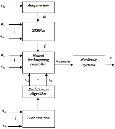
[image:3.595.323.545.331.580.2]The architecture of proposed evolutionary algorithm to compute the optimal parameters of GRBABC for nonlinear systems is shown in Fig.1.
Figure 1. proposed evolutionary algorithm to compute the optimal parameters of GRBABC for nonlinear systemsThe evolutionary algorithms which are described in the previous section are applied to search the optimal parameters c c1 2, ,...,cn called design parameters in section 2. This is to guarantee the stability of systems by ensuring negativity of the Lyapunov function and having a suitable time response.
The fitness function which is used for minimizing the evolutionary algorithms, described in the previous section, is defined as:
2 1
1 ( ) 2 n
i i
f e t
=
Table I. GA parameters
Parameters values
Size Population 20
Maximum of generation 1000
Prob. Crossover 0.2
Prob. Mutation 0.01
i
c search interval 150]
Table II. PSO parameters
Parameters values
Size Population 20
Maximum of generation 1000 i
c search interval (0 150]
5. Simulation Results
In this section, the proposed technique is applied to control two nonlinear chaotic systems: a Duffing Oscillator system (Example-1) and a Lü system (Example-2). It should be emphasized that development of the GRBABC does not require the knowledge of the system dynamic function and also, the design parameters are set via evolutionary algorithms.
5.1. Example (1): Duffing Oscillator System
Consider a second-order chaotic system such as well known Duffing's equation describing a special nonlinear circuit or a pendulum moving in a viscous medium under control [11]:
3
1 2 cos( ) ( , )
x= −px p x p x− − +q
ω
t u f x x u+ = + (26)
where p p p, ,1 2 and q are real constants. t is the time
variable and
ω
is the frequency. f x x( , ) is the systemdynamic function where
1 2
0.4, 1.1, 1.0, 1.8
p= p = − p = ω= and q=7 . u is the control effort.
The system dynamic function would be online estimated by the GRBFNN identifier. A GRBFNN identifier with five hidden nodes is utilized to approach the system dynamic function of the chaotic system.
The trajectory command is set as xd =cos( )t . The performance index I is defined as 2 2
1 2
I= e +e . The
performance index I is shown that the proposed method can achieve the favorable tracking performance.
The optimal parameters, minimum of fitness function and time of reach obtained via GA are shown in Table III.
Table III. Optimization results based on GA algorithm
C1 C2 Min f Treach (sec)
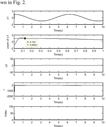
GA 26.9795 98.4360 5.7614×10⁻⁵ 0.124 The simulation results of GRBABC using optimal parameters obtained via GA for Duffing oscillator system are
shown in Fig. 2.
Figure 2. simulation results of Duffing oscillator system using optimal parameters obtained via GA.
The optimal parameters, minimum of fitness function and time of reach obtained via PSO are shown in Table IV.
Table IV. Optimization results based on PSO
C1 C2 Min f Treach (sec) PSO 18.7952 99.2720 5.7045×10⁻⁵ 0.102
[image:4.595.328.539.489.726.2]The simulation results of GRBABC using optimal parameters obtained via PSO for Duffing oscillator system are shown in Fig. 3.
Figure 3. simulation results of Duffing oscillator system using optimal parameters obtained via PSO.
0 1 2 3 4 5 6 7 8 9 10
-2 0 2
Time(s)
x1
0 0.1 0.2 0.3 0.4 0.5 0.6 0.7 0.8 0.9 1
-2 0 2
X: 0.124 Y: 0.9923
Time(s)
zoom
of
x
1
0 1 2 3 4 5 6 7 8 9 10
-50 0 50
Time(s)
x2
0 1 2 3 4 5 6 7 8 9 10
0 50 100
Time(s)
Index
0 1 2 3 4 5 6 7 8 9 10
-2000 -1000 0
Time(s)
u
0 1 2 3 4 5 6 7 8 9 10
-2 0 2
Time(s)
x1
0 0.1 0.2 0.3 0.4 0.5 0.6 0.7 0.8 0.9 1
-2 0 2
X: 0.102 Y: 0.9948
Time(s)
z
oom
of
x
1
0 1 2 3 4 5 6 7 8 9 10
-50 0 50
Time(s)
x2
0 1 2 3 4 5 6 7 8 9 10
0 20 40
Time(s)
Index
0 1 2 3 4 5 6 7 8 9 10
-600 -400 -2000 200
Time(s)
Figure 2 and Figure 3 show that the results have good performance compared with other papers like [7] and [11]. These results are converged to desirable trajectory command before 0.2 sec. However, the results of other papers are converged to that desirable trajectory command in 4sec.
5.2. Example (2): Lü System
Consider a third -order chaotic system such as well known Lü equation describing in [12]:
1 2 1
2 1 3 2
2 1 3 2
(
)
x
a x
x
x
x x cx
x
x x cx
=
−
= −
+
= −
+
(27)wherea=36, b=3, c=20 and uis the control effort. The system (27) can be rewritten as the following:
1 2
2
3 1 2 3
3
( , , )
x
x
x
x
x
f x x x
U
=
=
=
+
(28)and
2 1 2 3 1 1 2 2 3 1 3 4 2 3 5 1 2
( , , )
f x x x =a x a x+ +a x x +a x x +a x x (29) where a1= −46656 , a2=35136 , a3=1980 , a4= −1296 and
5 36
a = − . U is as the following
5 1
U a x u= (30)
The system dynamic function would be online estimated by the GRBFNN identifier. A GRBFNN identifier with five hidden nodes is utilized to approach the system dynamic function of the chaotic system.
The trajectory command is set as xd=cos( )t . The performance index I is defined as 2 2 2
1 2 3
I= e +e +e .
The performance index I shows that the proposed method can achieve favorable tracking performance.
The optimal parameters, minimum of fitness function and time of reach obtained via GA are shown in Table V.
Table V. Optimization results based on GA algorithm
C1 C2 C3 Min f Treach (sec)
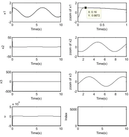
GA 42.2345 66.0835 68.0384 6.5943 10× −5 0.16
[image:5.595.177.432.440.710.2]The simulation results of GRBABC using optimal parameters obtained via GA for Lü system are shown in Fig. 4.
Figure 4. simulation results of Lü system using optimal parameters obtained via GA.
The optimal parameters, minimum of fitness function and time of reach which are obtained based on the PSO are shown in Table VI.
0 5 10
-2 0 2
Time(s)
x1
0 0.5 1
-2 0 2
X: 0.16 Y: 0.9872
Time(s)
zoom
of
x
1
0 5 10
-50 0 50
Time(s)
x2
2 4 6 8 10
-2 0 2
Time(s)
zoom
of
x
2
0 5 10
-500 0 500
Time(s)
x3
2 4 6 8 10
-2 0 2
Time(s)
zoom
of
x
3
0 5 10
-5 0 5x 10
6
Time(s)
u
0 5 10
0 5000
Time(s)
Table VI. Optimization results based on PSO
C1 C2 C3 Min f Treach (sec)
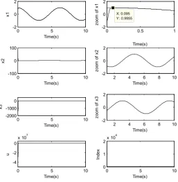
PSO 106.0333 82.2834 141.7942 1.2390×10⁻⁶ 0.095
[image:6.595.178.436.162.427.2]The simulation results of GRBABC using optimal parameters obtained via PSO for Lü system are shown in Fig. 5.
Figure 5. simulation results of Lü system using optimal parameters obtained via PSO.
Figure 4 and Figure 5 show that the results have good performance compared with other papers like [7], [12].
These results are converged to desirable trajectory command before 0.2 sec. However, the results of other papers are converged to that desirable trajectory command in 2sec.
6. Conclusion
In this paper, evolutionary algorithms are proposed to compute the optimal parameters of GRBABC for chaotic systems. The GA and PSO algorithms are used for finding the optimal parameters which minimize a cost function defined as the Lyapunov function. Design parameters are chosen based on the evolutionary algorithms, so the stability can be obtained when the parameters are appropriately selected. The proposed technique has been successfully applied to Duffing oscillator system and Lü like system. Simulation results verify that these proposed methods can achieve the favorable tracking performance.
REFERENCES
[1] G. Chen, “Controlling Chaos and Bifurcations in Engineering Systems”, Boca Raton, FL: CRC Press, 1999.
[2] E. Ott, C. Grebogi and JA. Yorke, “Controlling chaos”, Phys Rev Lett, Vol.64, pp.1196-1199, 1990.
[3] T. Zhang, S. S. Ge, and C. C. Hang, “Adaptive neural network control for strict-feedback nonlinear systems using backstepping design,” Automatica, Vol. 36, pp. 1835–1846, 2000.
[4] J. Y. Choi and J. A. Farrell, “Adaptive observer backstepping control using neural networks,” IEEE Trans. Neural Netw., Vol. 12, No. 5, pp.1103–1112, 2001.
[5] O. Kuljaca, N. Swamy,F.L.Lewis, and C.M.Kwan, “Design and implementation of industrial neural network controller using backstepping,” IEEE Trans. Ind. Electron., Vol. 50, No. 1, pp. 193–201, 2003.
[6] C. M. Lin and C. F. Hsu, “Recurrent-neural-network-based adaptive backstepping control for induction servomotor,” IEEE Trans. Ind. Electron., Vol. 52, No. 6, pp. 1677–1684, 2005.
[7] F. Farivar, M. Aliyari, M. A. Nekoui, M. Teshnehlab, “Gaussian Radial Basis Adaptive Backstepping Control for a Class of Nonlinear Systems”, Journal of Applied Sciences, Vol.9, No.2, pp.284-257, 2009.
[8] L. Wang, “Intelligent Optimization algorithms with
0 5 10
-2 0 2
Time(s)
x1
0 0.5 1
-2 0 2
X: 0.095 Y: 0.9955
zoom
of
x
1
Time(s)
0 5 10
-100 0 100
Time(s)
x2
2 4 6 8 10
-2 0 2
Time(s)
zoom
of
x
2
0 5 10
-2000 -1000 0
Time(s)
x3
2 4 6 8 10
-2 0 2
Time(s)
zoom
of
x
3
0 5 10
-4 -2
0x 10 7
Time(s)
u
0 5 10
0 1 2x 10
4
Time(s)
applications”, Beijing: Tsinghua University & Springer Press; 2001.
[9] B. Liu, L. Wang, YH. Jin, DX. Huang, “Advanced in particle swarm optimization algorithm”, Control Instrum Chem Ind, Vol.3, pp. 1-6, 2005.
[10] J. Kennedy, R. Eberhart, “Particle Swarm Optimization”, IEEE International Conference on Neural Networks, Vol.4, pp.1942-1948, 1995.
[11] K. Y. Lian, P. Liu, T. S. Chiang, and C. S. Chiu, “Adaptive synchronization design for chaotic systems via a scalar driving signal,” IEEE Trans. Circuits Syst. I, Fundam. Theory Appl., Vol. 49, No. 1, pp. 17–27, Jan. 2002.