What Drives the Dynamic Conditional Correlation of Foreign Exchange and Equity Returns?

(1)

Munich Personal RePEc Archive

What Drives the Dynamic Conditional

Correlation of Foreign Exchange and

Equity Returns?

Vargas, Gregorio A.

February 2008

Online at

https://mpra.ub.uni-muenchen.de/8027/

(2)

What Drives the Dynamic Conditional Correlation

of Foreign Exchange and Equity Returns?

Gregorio A. Vargas§ School of Economics Singapore Management University

First Version: 15 February 2008 This Version: 01 April 2008

Abstract

This paper establishes the link of microstructure and macroeconomic factors with the

time-varying conditional correlation of foreign exchange and excess equity returns. By using the

proposed DCC model with exogenous variables, capital flows and interest rate differentials are

shown to be significant determinants of this correlation which is inclusive of the short-run

variation of both asset returns. The results also provide evidence of the dynamic behavior of

global investors as they seek parity in equity returns between home and foreign markets to

reduce exchange rate risks.

JEL: C32, F31, G15

Key words: uncovered equity parity, order flow, ADCCX

(3)

1. Introduction

Short-run dynamics of nominal exchange rates are difficult to predict using

macroeconomic models. Meese and Rogoff (1983a, 1983b) and Rogoff (2001) and the survey of

the literature by Frankel and Rose (1995) have shown the failure of these models to capture the

behavior of exchange rates in short horizons. However, the recent shift from macroeconomic to

microstructure approach gave rise to more plausible models that can account for a large

proportion of the variations in the movement of exchange rates. In microstructure models of

exchange rates, Evans and Lyons (2002a, 2002b) revealed that order flow can explain 45% to

78% of the variation of the daily returns of the most liquid currencies. It is defined by Evans and

Lyons (2002a) as a measure of buying and selling pressure or simply the difference between

buyer-initiated and seller-initiated trade.

Related to order flow is the movement of equities across financial markets. Hau and Rey

(2004) showed that equity flows have grown from 4% of GDP for 1975 in the United States (US)

to 245% of the GDP in 2000 and argued that this movement in equity significantly influences the

short-run dynamics of foreign exchange balances. In this interaction between equity and

exchange rate, Brooks, et al. (2001) observed that there is a negative correlation between foreign

exchange return and excess equity return.

Hau and Rey (2006) referred to this phenomenon of negative correlation as uncovered

equity parity. They explained that home equity return in excess of foreign equity return

corresponds to the depreciation of the home currency. The depreciation is driven by domestic

purchases of foreign equities to reduce exchange rate risks. Under complete market assumption

this risk can be hedged and eliminated but Levich, et al. (1999) found that only a small fraction

of institutional investors actually hedge exchange rate risks so Hau and Rey (2004, 2006)

concluded that although the foreign exchange market is very liquid there are limits to the foreign

exchange arbitrage trading that investors may conduct in a complete market setting.

They also provided a plausible explanation to how equity and exchange returns relate to

each other in integrated financial markets using portfolio shifts. Changes in asset allocation

produce capital flows that find their way to the foreign exchange market. They also argued that

exchange rates are primarily a function of investment flows resulting from limited forex

arbitrage of risk-averse speculators. Furthermore, they posited that portfolio rebalancing moves

(4)

structure between foreign exchange return and excess equity return is constant, although they did

consider a structural change in the correlation between two periods.

In the new micro exchange rate economics using microstructure theory, Evans and Lyons

(2002a) demonstrated that foreign exchange order flow and the exchange rate are not

endogenous although both are simultaneously determined. They found that the innovations in

the exchange rate are driven largely by order flow but not the other way. This phenomenon

supports what they called pressure hypothesis where the causality goes from order flow to

exchange rates. This observed dynamics are consistent with the theoretical models of Glosten

and Milgrom (1985) and Kyle (1985) and the empirical investigation of Evans and Lyons

(2002b, 2006), Payne (2003) and Froot and Ramadorai (2005) where order flows provide

information about payoffs and they therefore drive prices.

Obstfeld and Rogoff (2000) have observed that fundamentals fail to explain the

movement of exchange rates. However, Hau and Rey (2006) showed that correlation exists

between foreign exchange return and capital flows while Evans and Lyons (2002a, 2006) used

regression to show that order flows and interest rate differentials significantly impact the foreign

exchange return.

The dynamic conditional correlation (DCC) model of Engle (2002) and its extensions are

widely used in the volatility literature and some of its applications in finance have been made by

Manera, et al. (2006) on spot and forward oil price returns, Cappiello, et al. (2006) on

international bond and equity returns, Billio, et al. (2006) sectoral asset allocation, Lanza, et al.

(2006) on oil forward and future prices, Kuper and Lestano (2007) on stock markets and interest

rates, among others. Incorporating exogenous variables in the DCC models is very important in

evaluating potential determinants of time-varying conditional correlation between asset returns

and this direction was suggested by Hafner and Franses (2003), Cappiello, et al. (2006) and Feng

(2006).

This paper has two main contributions. First, an extension of the DCC model is proposed

by incorporating exogenous variables in the evolution of the time-varying correlation. And

second, using this DCC model, it is shown that the time-varying conditional correlation of the

foreign exchange and excess equity returns varies across time and is driven by capital flows and

interest rate differentials. The approach here differs largely from the problem currently being

(5)

regression is used to measure the impact of order flow on exchange rate returns like in Evans and

Lyons (2002a) and Dunne, et al. (2004), while this paper employs a conditional correlation

model with exogenous variables to link the impact of two relevant variables on the time-varying

correlation.

This paper is organized as follows. Section 2 presents the DCC model with exogenous

variables. Section 3 specifies the time-varying correlation model of foreign exchange and excess

equity returns. Section 4 discusses the data. Section 5 contains the results and discussion, and

Section 6 concludes.

2. Asymmetric DCC Model with Exogenous Variables

The DCC model of Engle (2002) has the following specification. Let yt be an N×1 vector of asset returns and a sigma algebra of information up to time , without loss of

generality

1

−

ℑ_t t−1

t

μ is assumed to be zero, so

t t t

y =μ +ε

t t

t H u

2 / 1

=

ε where u_t ~ N

( )

0,Ι (1)

1

|ℑt−

t

ε ~N(0,Ht).

The conditional covariance matrix Ht can be expressed as a function of the DCC,

(

ijt iit jjt

)

t t t

t DRD h h

H = = ρ _, _, _, (2)

1 * 1 *− −

= t t t

t Q QQ

R , where Qt diag

( )

qii,t

* ₌

(3)

where Qt evolves according to

(

−Α Α−Β Β

)

+Α ₋ *₋ Α+Β ₋₁Β

1 *

1 ') '

( ' '

'Q Q t t Qt

Q ε ε . (4)

This model was extended by Cappiello, et al. (2006) to include asymmetric effects, that is

evolves according to

t Q

(

−Α' Α−Β' Β−Γ' Γ

)

+Α'( − − ')Α+Β' −1Β+Γ'( −1 −1')Γ

* 1 *

1 t t t t

t Q n n

N Q

Q

Q ε ε (5)

which is the Asymmetric DCC (ADCC) model.

Here t ~ N

(

0,Rt is an

*

ε

)

N×1 vector of standardized residuals where 21

, , *

,

−

= _i_t _ii_t

t

i ε h

ε and

(

*

)

*

t t

t I

(6)

and Γ are N×N diagonal matrices where Α=diag

( )

α , Β=diag

( )

β and Γ=diag

( )

η . To ensure positive definiteness of Qt it is assumed that α, β and η are non-negative coefficients

satisfying α +β +δη<1 where δ is the maximum eigenvalue of

( )

2 1 2 1 ₋ − Q N

Q which was

derived by Cappiello, et al. (2006). Furthermore,

∑

= − = T t t t T Q 1 * * 1 '

ˆ _ε _ε _and

_∑

= − = T t t tn n T N 1 1 '

ˆ _{serve as}

estimators of Q and N, respectively.

In this paper, a model of ADCC which incorporates exogenous variables that drive the

time-varying conditional covariance is proposed. Let Xt be a p×1 vector of exogenous

variables, ξ be a p×1 vector of parameters and Κ be an N×N matrix that can either be an identity matrix or matrix of ones. The following specification for the proposed model has the

following evolution of Qt,

(

)

1 1 1 1

* 1 *

1 ') ' '( ') '

( ' '

' '

' Α−Β Β−Γ Γ−Κ +Α − − Α+Β −Β+Γ − − Γ+Κ − (6)

Α

− Q Q N X t t Qt nt nt Xt

Q ξ ε ε ξ

which is called ADCCX, where

∑

= − = T t t X T X 1 1

ˆ _{is the estimator of}_X _{. It can be easily shown}

that the ADCCX regresses to a DCCX model if η =0; to the ADCC model if ξ =0; and, to the

DCC model if η =0 and ξ =0.

To ensure the positive definiteness of Qt, Κ is set as an identity matrix. It is further

specified that ξ'=

(

ξ1 L ξp

)

' where

( )k k

k ξ

ξ = be ( )k ∈

( )

0,1

k

ξ . This condition on ξk,

however, might be very restrictive because it implies that the exogenous variables only drive the

conditional variances but not the conditional covariances where . However, since

the conditional correlation is equal to

t ii

q _, q_ij_,_t i≠ j

t ij

r_,

(

)

12 , , , − t jj t ii t

ij q q

q , it is still indirectly a function of the

exogenous variables. This restriction can be relaxed by setting Κ as a matrix of ones instead.

Another concern about having ( )k k

k ξ

ξ = is that it restricts the sign of the parameters to be

non-negative. This is very limited and does not allow for the exogenous variable to have a negative

impact on the conditional covariance Qt. A remedy would be to allow ξk to take on a positive

(7)

The maximum likelihood estimator of the ADCCX model is derived in the Appendix.

3. DCC Models of Foreign Exchange and Equity Returns

The indicator of uncovered equity parity is expected to be time-varying that is why a

model that accounts for the variation in the correlation of foreign exchange and equity returns is

necessary. This proposition is consistent with the dynamic behavior of investors when they react

to changes in the economic environment by shifting their portfolio allocations between two

markets. The ADCCX model in the previous section is used to model this time-varying

correlation and is specified as follows. Let

(

)

(

)

( )

t

h t f t t

t dE dS dS f Q

R − , *− = (7)

where Qt follows the evolution of the ADCCX model in Eq. (6) so that

di dK

N Q

Q

Q −Α' Α−Β' Β−Γ' Γ−Κξ₁ −Κξ₂

(

)

(

h

)

t f t h t f t t t t t

t Q n n dK dK d i i 1

* 1 2 * 1 1 1 1 1 1 * 1 *

1 ') ' '( ')

(

' ₋ ₋ Α+Β ₋Β+Γ ₋ ₋ Γ+Κ ₋ − ₋ +Κ ₋ − ₋

Α

+ ε ε ξ ξ . (8)

Excess equity return is the difference between foreign and home log stock market index

returns, . The foreign exchange return is the log return of where is in

foreign currency per home currency so that foreign currency’s appreciation against the home

currency means . Capital flows is the difference between the net foreign equity

purchases by home residents and the net home equity purchases by foreigners, .

Interest rate differential is the difference between the foreign and home interest rates.

The

h t f

t dS

dS *− dEt Et Et

0 > −dE_t

* h t f t dK dK − h t f t i

i *−

dK and di are equal to the mean of h* and

t f

t dK

dK −

(

h

)

t f

t i

i

d *− , respectively. Alternative models ADCC, DCC and DCCX follow from Eq. (8) by setting the appropriate parameters to

zero.

Following from the exogenous proposition about order flows by Evans and Lyons

(2002a, 2006) and Froot and Ramadorai (2005), capital flows is taken as exogenous and the sign

of the parameter ξ₁ is negative which indicates that capital flows move to satisfy the uncovered

equity parity proposition by Hau and Rey (2006). Under the assumption of perfect price

flexibility, the sign of the parameter ξ₂ is positive which implies that if the foreign interest rate

rises it makes the foreign assets more attractive than before resulting in excess foreign equity

(8)

4. Data

The excess equity return, foreign exchange rate return, and capital flow data were

sourced from the Princeton University website of Hélène Rey. The data included in this study

are those of Germany and the United Kingdom (UK), considered the largest and most liquid

equity and foreign exchange markets in Europe during the period under consideration, vis-à-vis

the United States (US). The home country refers to the US. The data consists of monthly

observations from January 1980 to December 2001 for a total of 264 observations.

In particular, is the difference between the log foreign stock market index

return and the log US stock market index return,

h t f

t dS

dS *−

0 >

−dE_t is the foreign currency’s appreciation

against the dollar, is the difference between the net foreign equity purchases by US

residents and the net US equity purchases by foreigners normalized by the average flows in the

past 12 months, and is defined as the difference between end-of-the-month yields of the

foreign and US interest rates. With UK and the US the spread is the difference between 3-month

T-bill yields which were downloaded from of the Bank of England and the US Federal Reserve

websites, respectively. The interest differential between Germany and the US is derived from

the 1-year T-bond yields, taken from EconStat.com.

*

h t f

t dK

dK −

h t f

t i

i *−

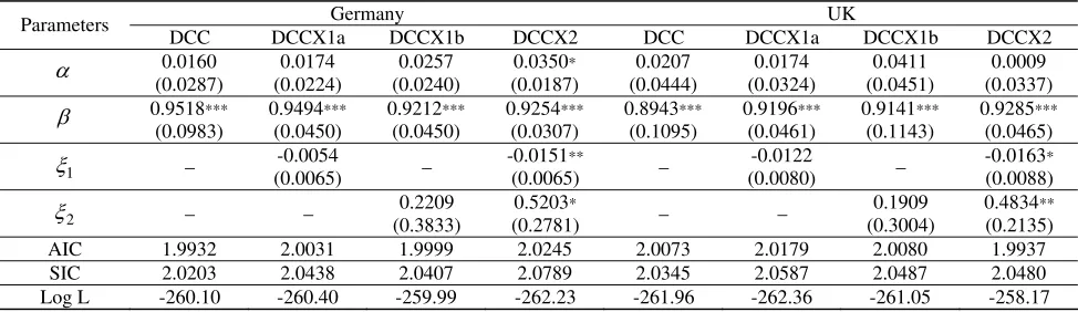
5. Results and Discussion

The results begin with the GARCH(1,1) model of the returns. Table 1 suggests that

foreign exchange returns exhibit heteroskedasticity based on the significant coefficients of the

GARCH models. These show that the pound and the mark demonstrate persistency in the

conditional variance even at the monthly returns. The volatility of excess equity returns is highly

persistent for British equities while German equities display large short-run shocks.

The initial DCC models are given in Table 2, these are the ADCC models for both

Germany and UK which indicate that there is no asymmetric effect between foreign exchange

and excess equity returns since η is not significant. The absence of asymmetric effect implies

that the magnitude of impact of either sign of the returns on the correlation does not significantly

(9)

the parameter estimates of the four models without asymmetric effect arising from the special

[image:9.612.155.452.153.238.2]

cases of Eq. (8).

Table 1. GARCH(1,1) Models of Foreign Exchange and Excess Equity Returns

Foreign Exchange Returns Excess Equity Returns Parameters

Germany UK Germany UK

# 0

a _(0.0010)0.0010 _(0.0002)0.0002 0.0230_(0.0095)** _(0.0018)0.0022

1 a 0.0214 (0.0340) 0.0696** (0.0338) 0.1707** (0.0833) 0.1266** (0.0577) 1

b 0.8853***

(0.1119) 0.9098*** (0.0398) 0.0000 (0.2908) 0.7103*** (0.1607) 0

[image:9.612.199.411.293.403.2]

a # is multiplied by a factor of 10

Table 2. ADCC Models of Foreign Exchange and Excess Equity Returns

Germany UK

α 0.0338

(0.0248)

0.0150 (0.0409)

β 0.9349***

(0.0569) 0.8790** (0.0810) η 0.0105 (0.0524) 0.0986 (0.0710)

AIC 2.0066 2.0133 SIC 2.0473 2.0540

Log L -260.86 -261.75

Table 3. DCC and DCCX Models of Foreign Exchange and Excess Equity Returns

Germany UK Parameters

DCC DCCX1a DCCX1b DCCX2 DCC DCCX1a DCCX1b DCCX2

α 0.0160 (0.0287) 0.0174 (0.0224) 0.0257 (0.0240) 0.0350* (0.0187) 0.0207 (0.0444) 0.0174 (0.0324) 0.0411 (0.0451) 0.0009 (0.0337)

β 0.9518***

(0.0983) 0.9494*** (0.0450) 0.9212*** (0.0450) 0.9254*** (0.0307) 0.8943*** (0.1095) 0.9196*** (0.0461) 0.9141*** (0.1143) 0.9285*** (0.0465) 1

ξ – -0.0054

(0.0065) –

-0.0151**

(0.0065) –

-0.0122

(0.0080) –

-0.0163*

(0.0088)

2

ξ – – 0.2209

(0.3833)

0.5203*

(0.2781) – –

0.1909 (0.3004)

0.4834**

(0.2135) AIC 1.9932 2.0031 1.9999 2.0245 2.0073 2.0179 2.0080 1.9937 SIC 2.0203 2.0438 2.0407 2.0789 2.0345 2.0587 2.0487 2.0480

Log L -260.10 -260.40 -259.99 -262.23 -261.96 -262.36 -261.05 -258.17

Note: Κ is a matrix of ones. The dKtf −dKth* and d⎜_⎝⎛itf*−ith⎞⎟_⎠ are stationary according to the Augmented Dickey-Fuller test in both cases.

The conditional correlation of foreign exchange and excess equity returns is highly

persistent as shown by the significant parameter estimates of the DCC models and indicates that

the correlation between the two is indeed time-varying for both markets. When only one of the

[image:9.612.67.554.440.581.2]

(10)

Both, however, are significant when they are in the model and the value of the parameter

estimates change drastically which signals model misspecification when either variable is

excluded. Although not reported here, the estimated asymmetric parameter of the ADCCX

model is also not significant for both cases.

The sign of the parameter estimates of capital flows, ξ₁, is correct and is significant in

both markets as shown by DCCX2. For the UK market the loglikelihood ratio test between the

DCC and the DCCX2 model is significant at the 10% level and confirms the hypothesis in the

literature that capital flows together with interest rate differentials significantly account for the

short-run dynamics of foreign exchange and excess equity returns. Figure 1 present the graphs

of the correlation. The graphs show that the inclusion of the exogenous variables clearly

accentuates the negative correlation and confirms the time-varying nature of the uncovered

equity parity.

Figure 1. DCC of the Mark (Pound) and the German (British) Excess Equity Returns v.v. the US

Germany UK

-.8 -.6 -.4 -.2 .0 .2 .4

1980 1985 1990 1995 2000

DCC

DCCX w ith X {dK}

DCCX w ith X {di} DCCX w ith X {dK, di}

-.8 -.6 -.4 -.2 .0 .2 .4

1980 1985 1990 1995 2000

DCC

DCCX w ith X {dK}

DCCX w ith X {di} DCCX w ith X {dK, di}

The outcome of this estimation shows that net capital flows from the home to the foreign

(11)

between the two markets when there is excess home equity return. This means that capital flows

act to bring equity returns to parity to reduce the exchange rate risk involved when either equity

markets have a higher return than the other through portfolio rebalancing according to Hau and

Rey (2004).

The parameter estimate of ξ₂ is positive and correctly signed and also significant in both

markets which confirms the result of Evans and Lyons (2002a, 2006). The relevance of interest

rates, in which inflation and growth expectations are imbedded, argues for the impact of

macroeconomic factors in driving this short-run dynamics of foreign exchange and equity

[image:11.612.213.516.415.680.2]

returns.

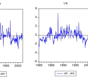
Figures 2 shows the net capital flows where a positive value indicates a move in net

capital towards Germany and UK, respectively, from the US. It is clear that when these graphs

are superimposed to Figures 1, respectively, the negative correlations are observed when net

capital flows are positive. And indeed, periods of heightened net capital outflow from the US

result in higher magnitudes of negative correlation. Similarly, Figure 3 reveals that when

Figure 2. Net Capital Flows of US Purchases of German (UK) Equities and German (UK) Purchases of US Equities

Germany UK

-6 -4 -2 0 2 4 6

1980 1985 1990 1995 2000

dKf - dKh*

-6 -4 -2 0 2 4 6

1980 1985 1990 1995 2000

(12)

Figure 3. Interest Rate Differential between Germany (UK) and the US, in percent

Germany UK

-.4 .0 .4 .8

1980 1985 1990 1995 2000

if* - ih d(if* - ih)

-.4 .0 .4 .8

1980 1985 1990 1995 2000

if* - ih d(if* - ih)

German and UK interest rates exceed the US interest rates, especially, in periods of large

positive differentials, the negative correlations are again observed to be correspondingly large.

These results are evidence of the changing dynamics of investor behavior as they respond

to varying risks in the two markets and they highlight the importance of equity return parity for

global investors as they seek to minimize the variance of their portfolio holdings. This dynamics

can be explained in the sense of the classic Markowitz’s efficient frontier. The significance of

the capital flows and interest rate differentials suggests that the correlation dynamics of foreign

exchange and excess equity returns are subject to both microstructure and macroeconomic

factors, at least in the sense of capital flows and interest rates, respectively.

6. Conclusion

The extension of the DCC model by incorporating exogenous variables is a natural

direction to take in order to identify the factors that drive the time-varying conditional correlation

of asset returns. By employing the DCC model, this paper shows that the correlation between

(13)

convenient tool for characterizing this time-varying correlation as a function of capital flows and

interest rate differentials.

The optimizing behavior of global investors shows that they seek equity parity to

minimize the foreign exchange risk in their portfolios. This paper demonstrates that this

behavior results in capital flow movements that adjust both the exchange rate and equity returns

in both home and foreign financial markets to satisfy uncovered equity parity. Capital flows

contain information about investor decisions, in the microstructure context, and is significant in

accounting for the time-varying conditional correlation of the foreign exchange and excess

equity returns. This confirms that investor behavior is a rich source of information that can

account for the short-run dynamics of foreign exchange rate. Furthermore, the interest rate

differentials represent macroeconomic information that arguably drives this correlation as well.

The results establish the link of microstructure and macroeconomic factors with the short-run

(14)

References

Billio M, Caporin M, Gobbo M. 2006. Flexible Dynamic Conditional Correlation Multivariate GARCH Models for Asset Allocation. Applied Financial Economics Letters. 2: 123-130.

Brooks R, Edison H, Kumar M, Sløk T. 2001. Exchange Rates and Capital Flows. IMF Working Paper WP/01/190, December.

Cappiello L, Engle R, Sheppard K. 2006. Asymmetric Dynamics in the Correlations of Global Equity and Bond Returns. Journal of Financial Econometrics4: 537-572.

Engle R. 2002. Dynamic Conditional Correlation: A Simple Class of Multivariate Generalized Autoregressive Conditional Heteroskedasticity Models. Journal of Business and Economic Statistics20: 339-350.

Engle R, Sheppard K. 2001. Theoretical and Empirical Properties of Dynamic Conditional Correlation Multivariate GARCH. NBER Working Paper 8554, October.

Evans M, Lyons R. 2002a. Order Flow and Exchange Rate Dynamics. Journal of Political Economy110: 170-180.

Evans M, Lyons R. 2002b. Informational Integration and FX Trading. Journal of International Money and Finance. 21: 807-831.

Evans M, Lyons R. 2006. Understanding Order Flow,” International Journal of Finance and Economics11: 3-23.

Feng Y. 2006. A Local Dynamic Conditional Correlation Model. Typescript, Heriot-Watt University, available at http://www.ma.hw.ac.uk/~yuanhua/papers/LDCC.pdf.

Froot K, Ramadorai T. 2005. Currency Returns, Intrinsic Value, and Institutional-Investor Flows. Journal of Finance60: 1535-1566.

Glosten L, Milgrom P. 1985. Bid, Ask, and Transaction Prices in a Specialist Market with Heterogeneously Informed Agents. Journal of Financial Economics14: 71-100.

Hafner C, Franses P. 2003. A Generalized Dynamic Conditional Correlation Model for Many Asset Returns. Typescript, Erasmus University Rotterdam, available at

http://www2.eur.nl/WebDOC/doc/econometrie/feweco20030708113101.pdf.

Hau H, Rey H. 2004. Can Portfolio Rebalancing Explain the Dynamics of Equity Returns, Equity Flows, and Exchange Rates? American Economic Review94: 126-133.

(15)

Kuper G, Lestano. 2007. Dynamic Conditional Correlation Analysis of Financial Market Interdependence: An Application to Thailand and Indonesia. Journal of Asian Economics18: 670-684.

Kyle A. 1985. Continuous Auctions and Insider Trading. Econometrica53: 1315-1335.

Lanza A, Manera M, McAleer M. 2006. Modeling Dynamic Conditional Correlations in WTI Oil Forward and Future Returns. Finance Research Letters3: 114-132.

Levich R, Hayt G, Ripston B. 1999. 1998 Survey of Derivative and Risk Management Practices by U.S. Institutional Investors. Survey conducted by the NYU Salomon Center, CIBC World Markets, and KPMG, available at http://pages.stern.nyu.edu/~rlevich/ wp/report-final.pdf.

Manera M, McAleer M, Grasso M. 2006. Modelling Time-Varying Conditional Correlations in the Volatility of Tapis Oil Spot and Forward Returns. Applied Financial Economics, 16: 525-533.

Meese R, Rogoff K. 1983a. Empirical Exchange Rate Models of the Seventies. Journal of International Economics14: 3-24.

Meese R, Rogoff K. 1983b. The Out-of-Sample Failure of Empirical Exchange Rate Models, in J Frenkel (ed.) Exchange Rate and International Macroeconomics. University of Chicago Press: Chicago.

Obstfeld M, Rogoff K. 2000. The Six Major Puzzles in International Macroeconomics: Is there a Common Cause? in B Bernanke and K Rogoff (eds.) NBER Macroeconomics Annual.

Cambridge MA.

(16)

APPENDIX

Maximum Likelihood Estimation of the ADCCX Model

The likelihood function under the assumption of multivariate normality of y_t is given by

( )

⎥⎥_⎦ ⎤ ⎢ ⎢ ⎣ ⎡ Π = − − = ' 2 1 1 1 2 1 2 1 ) |

( ytHt yt

t N T t t e H y L π θ .

Using the two-stage LIML procedure proposed by Engle (2002) the likelihood function is

maximized with respect to two sets of parameters in succeeding steps.

The vector θ consists of GARCH parameters for each element of the -dimensional

and the parameters of , where

N y_t

t

Q y_t =ε_t. Engle and Sheppard (2001) have shown the

consistency and asymptotic normality of this two-stage procedure. The loglikelihood function is

( )

(

)

∑

= − + + − = T t t t t t

t N H y H y

y L

1

1 2

1 log 2 log '

2 1 ) | , (

log θ θ π

( )

(

)

∑

= − − − + + + − = T t t t t t t t

t D y D R D y

R N 1 1 1 1 ' log 2 log 2 log 2 1 _π

where θ₁ consists of parameters of the MGARCH model, θ₂ consists of parameters of .

Furthermore, and

t Q

t t t

t DRD

H = D_t =diag

(

h₁₁1/_,2_tKh_NN1/2_,_t

)

. Engle and Sheppard (2001) set as the identity matrix in the first stage estimation,

t R

( )

(

)

∑

= − − − + + + − = T t t t N t t t N

t N I D y D I D y

y L 1 1 1 1

1 log 2 log 2log '

2 1 ) | (

log θ π

θˆ1 =argmax[logL(θ1| yt)]

which is equivalent to estimation of the univariate GARCH models of yt.

The second stage estimation involves

( )

(

)

∑

= − − − + + + − = T t t t t t t t t

t N R D y D R D y

y L 1 1 1 1 1

2 log 2 log 2log ˆ ' ˆ ˆ

2 1 ) , ˆ | (

log θ θ π

where t Dt yt. And since where

1 * = ˆ−

ε ₌ *−1 *−1

t t t

t Q QQ

R Q_t* =diag

( )

q_iit

( )

(

)

∑

= − − − − − ₊ ₊ + − = T t t t t t t t t t t

t N Q QQ D Q QQ

y L 1 * 1 1 * 1 * * 1 * 1 * 1

2 log2 log 2log ˆ '( )

2 1 ) , ˆ | (

(17)

The constant terms Nlog

( )

2π and 2logDˆt are not necessary in the maximization and

are dropped from the function so that

(

)

∑

= − − − − − ₊ − = T t t t t t t t t t

t Q QQ Q QQ

y L 1 * 1 1 * 1 * * 1 * 1 * 1

2 log '( )

2 1 ) , ˆ | ( '

log θ θ ε ε

θˆ2 =argmax[logL'(θ2 |θˆ1,yt)]. An expansion of the second stage loglikelihood function is

(

)

{

∑

= − − − − − − −

− ₊_Α _Α₊_Β _Β₊_Γ _Γ₊_Κ

− = T t t t t t t t t t

t Q Q Q n n X Q

y L 1 1 * 1 1 1 1 * 1 * 1 1 * 1

2 '( ') ' '( ') '

~ log 2 1 ) , ˆ | ( '

log θ θ ε ε ξ

(

)

(

* 1

)

1 *

}

1 1 1 1 * 1 * 1 1 * *' ' ) ' ( ' ' ) ' ( ' ~ t t t t t t t t t

t Q Q ε ε Q n n ξ X Q ε

ε − −

− − − − − −

− ₊_Α _Α₊_Β _Β₊_Γ _Γ₊_Κ

+

where

(

Q Q Q N X

)

Q~= −Α' Α−Β' Β−Γ' Γ−Κξ' and

1 1 1 1 * 1 *

1 ') ' '( ') '

( ' ~ − − − − −

− Α+Β Β+Γ Γ+Κ

Α +

= t t t t t t

t Q Q n n X

Q ε ε ξ .

The maximum likelihood estimators of ADCC, DCC and DCCX models can be derived