Design of a Robust Controller for Inverted Pendulum

(1)

Volume 112 – No 16, February 2015

Design of a Robust Controller for Inverted Pendulum

Arunesh Kumar Singh

, Ph.D

Electrical Engineering Department Jamia Millia Islamia, New Delhi

D.K.Chaturvedi

, Ph.D

Electrical Engineering Department Dayalbagh Educational Institute,

Agra

Nitin Kumar Pal

Electrical Engineering Department Jamia Millia Islamia, New Delhi

ABSTRACT

In this paper, robust controller is developed by using H∞ controller to improve the performance of the Invert Pendulum. In this paper, introduced a controller by combining the classical PID, the fuzzy controllers and H∞ controller and thus a new controller has been achieved. The simulations done on inverted pendulum using the new H∞ fuzzy PID controller provides better system responses in terms of transient and steady-state performances when compared to the pure classical PID or the pure fuzzy controller applications.

Keywords

Inverted Pendulum, PID Controller, Fuzzy Logic controller, H∞ controller.

1. INTRODUCTION

As a child, we try to balance a broom-stick on his index finger or the palm of his hand. We have to constantly adjust the position of the hand to keep the object upright. An inverted pendulum does basically the same thing. However, it is limited in that it only moves in one dimension, while our hand could move up, down, sideways, etc.

Just like the broom-stick, an Inverted Pendulum is an unstable system. Force must be properly applied to keep the system stable. To achieve this, proper control theory is required. The Inverted Pendulum is useful in evaluating and comparing of various nonlinear systems.

It is virtually impossible to balance a pendulum in the inverted position without applying some external force to the system. The Carriage Balanced Inverted Pendulum (CBIP) system, shown below Fig 1, allows this control force to be applied to the pendulum carriage. The outputs from the CBIP rig can be carriage position, carriage velocity, and pendulum angle and pendulum angular velocity. In the present work out of these only pendulum angle is considered as output.

Figure 1 Carriage Balanced Inverted Pendulum (CBIP)

2. INVERTED PENDULUM PROBLEM

FORMULATION

The following figure shows an inverted pendulum. The aim is to move the wagon along the x direction to a desired point without the pendulum falling. The wagons x position (not in our case) and the pendulum angle ϕ are measured and supplied to the control system. A disturbance force, FDISTURBANCE, can be applied on top of the pendulum.

A mathematical model of the system is developed, giving the angle of the pendulum resulting from a force applied to the base [2]. The Free Body Diagram of the system is used to obtain the equations of motion. Below are the two Free Body Diagrams of the system.

The physical parameters of the system prototype are tabulated as follows:

1. M Mass of the Cart 1.096Kg

2. m Mass of the Pendulum 0.109Kg

3. b Friction of the Cart 0.1 N/m/sec

4. L Length of pendulum to Center of mass 0.25 m

5. I Moment of Inertia (Pendulum)01.0034Kg-m2

6. F Force applied to the cart

7. x Cart Position Coordinate

8. ϕ Pendulum Angle from vertical

9. θ Pendulum angle from the vertical downwards

Putting the parameters and find Transfer function of the Inverted Pendulum

2

( )

0.02725

( )

0.0102125

0.26705

s

X s

s



_



3 2

( )

2.35655

( )

0.00883167

27.9169

2.30942

s

U s

s



_

(2)

Volume 112 – No 16, February 2015 Since the system pole is right hand side so it is an unstable

system. We can see it with the help of step response and impulse response also.

3. PID CONTROLLER

The PID controller is the most common form of feedback. It was an essential element of early governors and it became the standard tool when process control emerged in the 1940s. The PID controller calculation involves three separate parameters; the proportional, the integral and derivative values. The proportional value determines the reaction to the current error, the integral value determines the reaction based on the sum of recent errors, and the derivative value determines the reaction based on the rate at which the error has been changing. The weighted sum of these three actions is used to adjust the process via a control element such as the position of a control valve or the power supply of a heating element. . Note that the use of the PID algorithm for control does not guarantee optimal control of the system or system stability [9] [11].

The PID control scheme is named after its three correcting terms, whose sum constitutes the manipulated variable (MV)

[image:2.595.317.559.111.187.2]

[11]. Hence MV (t) =

P

_out+

I

_out+

D

_out

Fig. 2 A block diagram of a PID controller

Where, P_out,

I

_out,

D

_out are the contributions to the output

from the PID controller from each of the three terms.

If the PID controller parameters (the gains of the proportional, integral and derivative terms) are chosen incorrectly, the controlled process input can be unstable, i.e. its output diverges, with or without oscillation, and is limited only by saturation or mechanical breakage. Tuning a control loop is the adjustment of its control parameters (gain/proportional band, integral gain/reset, derivative gain/rate) to the optimum values for the desired control response [10].

There are several methods for tuning a PID loop. The most effective methods generally involve the development of some form of process model, and then choosing P, I, and D based on the dynamic model parameters. Manual tuning methods can be relatively inefficient.

4. FUZZY LOGIC CONTROL

Fuzzy concepts derive from fuzzy phenomena that commonly occur in the natural world. The concepts formed in human brains for perceiving, recognizing, and categorizing natural phenomena are often fuzzy concepts. An objective of fuzzy logic has been to make computers think like people. Boundaries of these concepts are vague. We will introduce the basic concept of fuzzy systems and control in this chapter.

A specific type of knowledge-based control is the fuzzy rule-based control, where the control actions corresponding to particular conditions of the system are described in terms of fuzzy if-then rules. Fuzzy sets are used to define the meaning of qualitative values of the controller inputs and outputs.

Figure 3 shows the basic structure of a fuzzy logic controller. The main building units of an FLC are a fuzzification unit, a

fuzzy logic inference unit, a rule-base, and a defuzzification unit. Defuzzification is the process of converting inferred fuzzy control actions into a crisp control action.

Figure 3: Basic structure of a Fuzzy Logic Controller

Fuzzy logic controllers are used to improve the performance. In the case of highly complex systems, fuzzy logic could be the only solution.

5. ROBUST CONTROL

Conventional controllers can make the system stable under certain conditions i.e need of accurate mathematical model(without uncertainty).However in actual system due to presence of noise and disturbances and parameter uncertainties so application of control law to these kind of system becomes difficult. In order to solve such type of problems, various robust control techniques such as H∞ [19-22,], QFT and sliding mode control ,Internal model control etc. While going through various literature survey, it is

observed that H_ technique is widely used in various control applications and it is found that H∞ technique can deal with the problems in a better way as compared to its analogue counterparts.

The foundations on which the H∞ control is laid are discussed in depth to offer more clarity on the methodology of this robust control method. The foundations in question are linear fractional transformations(LFT’s) and structured singular values(μ)[12].These two concepts help analyze the effect of uncertain models on achievable closed-loop performance and ultimately design a controller that provides the optimal-worst case performance in the face of the plant uncertainty. The basic idea in modeling an uncertain system is to separate what is known from what is unknown in a feedback-like connection , and bound the possible values of the unknown elements.

6. SIMULATION AND RESULTS

[image:2.595.54.288.317.413.2]

In this paper, the mathematical model and equations using the transfer function of the inverted pendulum have been determined. By implementing all these equations into MATLAB M-file command, and simulate it in MATLAB SIMULATION. The following Open Loop and closed loop SIMULATION of system are shown in Fig (4) and Fig (5).

Fig.4 Open- Loop Inverted Pendulum System

Fig.5 Closed Loop Inverted Pendulum System

The Open and closed loop response of Inverted Pendulum is shown in following Figure (6) to Figure (9), it can be noticed that the inverted pendulum system is not stable without

2.35655s den(s) Transfer Fcn

Step Scope2

2.35655s den(s) Transfer Fcn

[image:2.595.317.534.608.720.2]

(3)

Volume 112 – No 16, February 2015 controller. The curve of the pendulum’s angle was approached

infinity as the time increases.

[image:3.595.320.536.74.190.2]

Fig. 6 Impulse Response of Open loop Inverted Pendulum

[image:3.595.59.274.106.249.2]

Fig. 7 Step Response of Open loop Inverted Pendulum

Fig.8 Impulse Response of Closed loop Inverted Pendulum

Fig.9 Step Response of Closed loop Inverted Pendulum

6.1 PID Control Method

The implementation of PID control method is done by adjusting the value of gain K, Ki, and Kd in order to get the best response of the system. SIMULATION of Inverted pendulum with PID controller is shown in bellow Fig (10).

Fig.10 Simulation of Inverted Pendulum using PID Controller

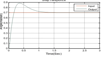
Step response of pendulum angle with PID controller is shown in bellow Fig (11).With PID controller the system controlled but it settling time as well as the rise time and max. Overshoot is high.

Fig.11 Step Response of pendulum angle with PID

6.2 Fuzzy Logic Control Method

Figure (12) show the simulation of Fuzzy Logic Controller.

Fig.12 Simulation of Inverted Pendulum using Fuzzy Logic Controller

[image:3.595.317.528.273.395.2]

If we give a external impulse signal as a disturbance to the system then the system become more unstable. The SIMULATION of FLC with external disturbance is shown in bellow Fig (13).

Fig.13 Simulation of Inverted Pendulum with Impulse Disturbance

0 0.5 1 1.5 2 2.5 3

0 2000 4000 6000 8000 10000 12000 14000 16000 18000

Time(Sec)

A

n

g

le

(R

a

d

ia

n

)

Impulse Responce

Output

0 0.5 1 1.5 2 2.5 3

0 0.5 1 1.5 2 2.5x 10

Time(Sec)

A

ng

le

(R

ad

ia

n)

Step Responce

Output

0 0.5 1 1.5 2 2.5 3 0

1000 2000 3000 4000 5000 6000 7000 8000 9000

Time(Sec)

An

gl

e(

Ra

di

an

)

Impulse Responce

Output

0 0.5 1 1.5 2 2.5 3

0 2 4 6 8 10 12 14x 10

Time(Sec)

A

ng

le

(R

ad

ia

n)

Step Responce

Output

Transfer Fcn 2.35655 s

den (s) Step

Scope 6

Scope 2 PID Controller

PID

0 0.5 1 1.5 2 2.5 3 0

0.1 0.2 0.3 0.4 0.5 0.6 0.7 0.8 0.9

Time(Sec)

A

ng

le

(R

ad

ia

n)

Step Responce

Input Output

Transfer Fcn 2.35655 s den (s) Step

Scope 6 _{Scope 3}

Scope 2 Gain 4

K- Gain 2 -K-Fuzzy Logic

Controller Error Dot

du /dt Error

-K-2.35655s den(s)

Transfer Fcn Scope2 Impulse Disturbance

-K-Gain4

-K-Gain3

-K-Gain2

Fuzzy Logic Controller

du/dt Derivative 0

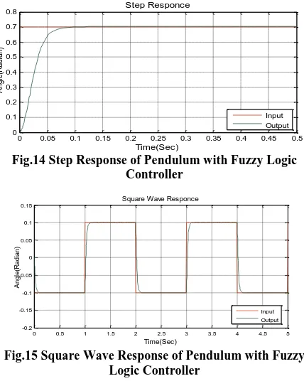
[image:3.595.314.543.444.546.2] [image:3.595.319.536.634.722.2]

(4)

Volume 112 – No 16, February 2015 Step response of pendulum with FLC is shown in Fig (14).

[image:4.595.316.542.115.213.2]

From bellow figure it is clearly seen that with FLC we get better response in term of settling time, overshoot and rise time is better. Square wave response of inverted pendulum with fuzzy logic controller is shown in fig. (15)

Fig.14 Step Response of Pendulum with Fuzzy Logic Controller

Fig.15 Square Wave Response of Pendulum with Fuzzy Logic Controller

Figure (17) shows the response of inverted pendulum with fuzzy Logic Controller while an external disturbance applied on the system.

Fig.17 Response of Pendulum with Impulse Disturbance

6.3 Robust

Control with Fuzzy Logic

Controller

Figure (18) show the simulation of Robust control (H∞) with Fuzzy Logic. For designing Robust controller (H ∞ Controller) used m-file coding and find out controller value in the form of numerator and denominator.

The SIMULATION of Robust Controller (H∞ Controller) with FLC and impulse signal given to the system as a disturbance shown in bellow Fig (19).

[image:4.595.60.274.133.401.2]

Figure (20) shows the step response of inverted pendulum with H∞ controller Using FLC. Square wave response of inverted pendulum with H∞ using fuzzy logic controller is shown in Fig. (21).

[image:4.595.316.531.300.562.2]

Fig. 20 Step Response of Pendulum with H∞ and Fuzzy Logic Controller

Fig.21 Square Wave Response of Pendulum with H∞ and Fuzzy Logic Controller

[image:4.595.57.277.443.541.2]

Figure (22) shows the response of inverted pendulum with H∞ fuzzy Logic Controller while an external disturbance applied on the system.

Fig.22 Response of Pendulum with Impulse Disturbance

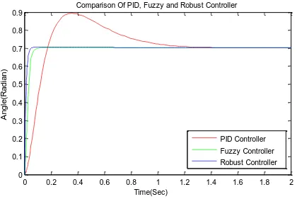
6.4 Comparison of Various Controllers

The performance of various controllers for third order process has been compared in the table 1 and Fig. (23). It can be seen

0 0.05 0.1 0.15 0.2 0.25 0.3 0.35 0.4 0.45 0.5 0 0.1 0.2 0.3 0.4 0.5 0.6 0.7 0.8 Time(Sec) A ng le (R ad ia n) Step Responce Input Output

0 0.5 1 1.5 2 2.5 3 3.5 4 4.5 5

-0.2 -0.15 -0.1 -0.05 0 0.05 0.1 0.15 Time(Sec) A n g le (R a d ia n )

Square Wave Responce

Input Output

0 0.05 0.1 0.15 0.2 0.25 0.3 0.35 0 0.2 0.4 0.6 0.8 1 1.2x 10

Time(Sec) A ng le (R ad ia n) Impulse Disturbance Output 2.35655s den(s) Transfer Fcn Step Scope2 den(s) 1000*[ 0.0467 0.4623 1.1553 0.0924]

Robust Controller -K-Gain4 -K-Gain3 -K-Gain2 Fuzzy Logic Controller du/dt Error Dot 2.35655s den(s) Transfer Fcn Scope2

den(s) 1000*[ 0.0467 0.4623 1.1553 0.0924]

Robust Control Impulse Disturbance -K-Gain3 -K-Gain2 Fuzzy Logic Controller du/dt Error Dot 0 Constant -K-.

0 0.05 0.1 0.15 0.2 0.25 0.3 0.35 0.4 0.45 0.5 0 0.1 0.2 0.3 0.4 0.5 0.6 0.7 0.8 Time(Sec) An gl e( R ad ia n) Step Responce Input Output

0 0.5 1 1.5 2 2.5 3 3.5 4 4.5 5 -0.2 -0.15 -0.1 -0.05 0 0.05 0.1 0.15 Time(Sec) A n g le (R a d ia n )

Square Wave Responce

Input Output

0 0.05 0.1 0.15 0.2 0.25 0.3 0.35 -2 0 2 4 6 8 10 12 14x 10

[image:4.595.315.532.603.715.2] [image:4.595.59.276.657.718.2]

(5)

Volume 112 – No 16, February 2015 that both controllers, fuzzy and robust controller (H∞) have

performed better than conventional controllers for Inverted Pendulum systems. However, the robust control using fuzzy logic controller has slightly better performance than Fuzzy PD controller in terms of rise time and settling time.

[image:5.595.67.277.132.276.2]

Fig. 23 Comparison of various controllers

Table 1: Performance Indices of various Controllers

Contro ller Type

Performance Index

Rise Time Tr (Sec.)

Max. Overshoot Mp (%)

Settling Time Ts (Sec.)

Steady State Error (Ess) Conv.

PID

0.1745 0.8937 1.5 0.7024

FLC 0.106 0.705 0.17 0.7034

H∞ using FLC

0.05 0.7065 0.105 0.7034

7. CONCLUSION

Modeling and robust control design of nonlinear system is investigated in this thesis. This thesis also presented an overview of working with H∞ (Robust control method) of designing controllers. Although the application of H∞ requires understanding of the linear algebra and intricate mathematics therefore the aim of this thesis to give a clear picture of the working procedure and how to apply it to practical problems in hand.

The model used in this paper is nonlinear in nature and are linearized using standard linearizing methods. Using this model, a set of transfer functions are derived which show the dynamics of the system. The same model is used to design various controller such as conventional PID controller, Fuzzy Logic Controller and H∞ Controller and comparative study of the performance is done in the face of model uncertainties, disturbances, rise time, settling time, maximum overshoot and finally we conclude that robust control using fuzzy Logic Controller is best controller compared to conventional and fuzzy controller.

8. REFERENCE

[1] J. Lam, “Control of an Inverted Pendulum”, University of California, Santa Barbara, 10 June 2004.

[2] Yanmei Liu and Zhen Chen, Dingy Xue, Xinhe Xu “Real-Time Controlling of Inverted Pendulum by Fuzzy” Proceedings of the IEEE International Conference on Automation and Logistics Shenyang, China August 2009

[3] Shiriaev A.S., Friesel A., Perram J. “On Stabilization of Rotational Modes of an Inverted Pendulum” Proceedings of the 39th IEEE Conference on Decision and Control Sydney, Australia December, 2000

[4] R. Ooi, “Balancing a Two-Wheeled Autonomous Robot”, University of Western Australia, 3 Nov. 2003.

[5] Marzi Hosein, “Fuzzy Control of an Inverted Pendulum using AC Induction Motor Actuator” IEEE International Conference on Computational Intelligence for Measurement Systems and Applications La Coruna - Spain, July 2006

[6] Marius L. Tomescu, “An Algorithm for Stability of Takagi–Sugeno Fuzzy Logic Controller”, Proceedings of 3rd Romanian Hungarian joint symposium on applied computational intelligence, SACI 2006 Timisoara, Romania may 2006

[7] Songmoung Nundrakwang, Taworn Benjanarasuth, Jongkol Ngamwiwit and Noriyuki Komine, “Hybrid Controller for Swinging up Inverted Pendulum System”, ELITE, CMS, 2005

[8] Robert A. Paz “The Design of the PID Controller” Klipsch School of Electrical and Computer Engineering June 12, 2001.

[9] Katsuhiko Ogata “Modern control Engineering” university of Minnesota, prentice hall, Upper Saddle River. New Jersey 07458

[11]Theory of Robust Control by Carsten Scherer Mechanical Engineering Systems and Control Group Delft University of Technology the Netherlands

[13]Yasunobu Seiji and Yamasaki Hiroaki, “Evolutionary Control Method and Swing Up and Stabilization Control of Inverted Pendulum”, Joint 9th IFSA World Congress and

[14]Stonier R.J. and Young N., “Co-evolutionary learning and hierarchical fuzzy control for the inverted pendulum”, The Congress on Evolutionary Computation, CEC, 2003, volume 1, Page 467-473

[15]Ben M. Chen, Robust and H∞ Control, Springer-Verlag, 2000.

[16]Sunjie Zhang, Zidong Wang, Derui Ding, and Huisheng Shu “H∞ Fuzzy Control With Randomly Occurring Infinite Distributed Delays and Channel Fadings” IEEE Transactions On Fuzzy Systems, Vol. 22, No. 1, February 2014

[17]Baohua Wang and Yongfei Zhang “Design for H∞ Excitation Controller Based on Fuzzy T-S Model” Ieee Transactions 2010.

[18]Li-Ying Sun, Shaocheng Tong, and Yi Liu “Adaptive Backstepping Sliding Mode H∞ Control of Static Var Compensator” Ieee Transactions On Control Systems Technology, Vol. 19, No. 5, September 2011.

0 0.2 0.4 0.6 0.8 1 1.2 1.4 1.6 1.8 2

0 0.1 0.2 0.3 0.4 0.5 0.6 0.7 0.8 0.9

Time(Sec)

A

n

g

le

(R

a

d

ia

n

)

Comparison Of PID, Fuzzy and Robust Controller

(6)

Volume 112 – No 16, February 2015 [19]Ali Poorhossein and Ali Vahidian-Kamyad “Design and

implementation of Sugeno controller for Inverted Pendulum on a Cart system” IEEE 8th International Symposium on Intelligent Systems and Informatics • September 10-11, 2010, Subotica, Serbia

[20]Hosein Marzi “Fuzzy Control of an Inverted Pendulum using AC Induction Motor Actuator” IEEE International Conference on Computational Intelligence for Measurement Systems and Applications La Coruna - Spain, 12-14 July 2006

[21]Zhao Yang, Xiao Xiangning, Member, IEEE , Xudong Jia “Nonlinear PID Controller of H-Bridge Cascade SSSC Top Level Control” DRPT2008 6-9 April 2008 Nanjing China.

[22]Lin Wang, Shifu Zheng, Xinping Wang and Liping Fan “Fuzzy Control of a Double Inverted Pendulum Based on Information Fusion” International Conference on Intelligent Control and Information Processing August 13-15, 2010 - Dalian, China

[23]Meysam Ghanavati, Vahid Johari Majd and Malek Ghanavati “Control of Inverted Pendulum System by using a new Robust Model Predictive Control Strategy” 2011 International Siberian Conference on Control and Communications SIBCON.