The exp( j(x)) Method and Its Applications for Solving Some Nonlinear Evolution Equations in Mathematical Physics

(1)

http://dx.doi.org/10.4236/ajcm.2015.54041

( )

(

)

The

  

  

 _ _

 

exp

−

ϕ ξ

Method and Its Applications

for Solving Some Nonlinear Evolution

Equations in Mathematical Physics

Maha S. M. Shehata

Department of Mathematics, Faculty of Science, Zagazig University, Zagazig, Egypt

Received 23 January 2015; accepted 27 December 2015; published 30 December 2015

This work is licensed under the Creative Commons Attribution International License (CC BY). http://creativecommons.org/licenses/by/4.0/

Abstract

The exp

(

−ϕ ξ

( )

)

method is employed to find the exact traveling wave solutions involving

para-meters for nonlinear evolution equations. When these parapara-meters are taken to be special values, the solitary wave solutions are derived from the exact traveling wave solutions. It is shown that the exp

(

−ϕ ξ

( )

)

method provides an effective and a more powerful mathematical tool for solving

nonlinear evolution equations in mathematical physics. Comparison between our results and the well-known results will be presented.

Keywords

The exp

(

−ϕ ξ

( )

)

Method, (2+1)-Dimensional Soliton Breaking Equation, (3+1)-Dimensional

Kadomstev-Petviash-Vili, Traveling Wave Solutions, Solitary Wave Solutions

1. Introduction

(2)

series method [18], G

G

′    

 -expansion method [19]-[22], Jacobi elliptic function method [23]-[26], the

( )

(

)

exp −ϕ ξ -expansion method [27]-[29] and so on.

The objective of this article is to investigate more applications than obtained in [27]-[29] to justify and

demonstrate the advantages of the exp

(

−ϕ ξ

( )

)

method. Here, we apply this method to (2+1)-dimensional soliton breaking equation [30] and (3+1)-dimensional Kadomstev-Petviash-vili.

2. Description of Method

Consider the following nonlinear evolution equation

(

, ,_t _x, _tt, _xx,

)

0,

F u u u u u  = (1)

where F is a polynomial in u x t

( )

, and its partial derivatives in which the highest order derivatives and nonlinear terms are involved. In the following,we give the main steps of this method

Step 1. We use the wave transformation

( ) ( )

, , ,

u x t =u

ξ

= −x ct (2)

where c is a positive constant, to reduce Equation (1) to the following ODE:

(

, , , ,

)

0,

P u u u u′ ′′ ′′′ = (3)

where P is a polynomial in u

( )

ξ

and its total derivatives,while d d

' '

ξ = .

Step 2. Suppose that the solution of ODE (3) can be expressed by a polynomial in exp

(

−ϕ ξ

( )

)

as follows

( )

m

(

exp

(

( )

)

m , m 0,

u ξ =a −ϕ ξ + a ≠ (4)

where

ϕ ξ

( )

satisfies the ODE in the form

( )

exp

(

( )

)

exp

(

( )

)

,

ϕ ξ′ = −ϕ ξ +µ ϕ ξ +λ (5)

the solutions of ODE (5) are when

λ

2−4

µ

>0,

µ

≠0,

( )

(

)

2 2

1 4

4 tanh 2

ln ,

2

C

λ µ

λ µ ξ λ

ϕ ξ

µ

  ₋  

− −  + − 

 

 _ _ 

=  

 

 

(6)

when

λ

2−4

µ

>0,

µ

=0,

( )

₍

₎

1

ln ,

exp C 1

λ ϕ ξ

λ ξ

 

= − _ _

+ −

  (7)

when

λ

2−4

µ

=0,

µ

≠0,

λ

≠0,

( )

(

₍

1

)

₎

)

2 1

2 2

ln C ,

C

λ ξ ϕ ξ

λ ξ

 + + 

= _− _

+

  (8)

when

λ

2−4

µ

=0,

µ

=0,

λ

=0,

( )

ln

(

C1

)

,

ϕ ξ

=

ξ

+ (9)

(3)

( )

(

)

2 2

1 4

4 tan

2

ln ,

2

C

µ λ

µ λ ξ λ

ϕ ξ

µ

  ₋  

 −  + − 

 

 _ _ 

=  

 

 

(10)

where am,, ,λ µ are constants to be determined later,

Step 3. Substitute Equation (4) along Equation (5) into Equation (3) and collecting all the terms of the same power exp

(

−mϕ ξ

( )

)

, m=0,1, 2, 3, and equating them to zero, we obtain a system of algebraic equations, which can be solved by Maple or Mathematica to get the values of a_i.

Step 4. substituting these values and the solutions of Equation (5) into Equation (3) we obtain the exact solutions of Equation (1).

3. Application

Here, we will apply the exp

(

−ϕ ξ

( )

)

method described in Section 2 to find the exact traveling wave solutions and then the solitary wave slutions for the following nonlinear systems of evolution evolution equations.

3.1. Example 1: The (2+1)-Dimensional Breaking Soliton Equations

Let us consider the (2+1)-dimensional breaking soliton equations [30]:

4 4 0,

,

t xxy x x

y x

u u uv u v

u v

α α α

+ + + =

  =

 (11)

where

α

is known constant. Equation (11) describes the (2+1)-dimensional interaction of a Riemann wave propagating along the y-axis with along wave along the x-axis. In the past years, many authors have studied Equation (11). For instance, Zhang has successfully extended the generalized auxiliary equation method of the (2+1)-dimensional breaking soliton equations in [31]. Some soliton-like solutions were obtained by the generalized expansion of Riccati equation in [32]. Recently, a class of periodic wave solutions were obtained by the mapping method in [33]. Two classes of new exact solutions were obtained by the singular manifold method in [34].

Using the wave variable

ξ

= + −x y ct and proceeding as before we find

4 4 0,

,

cu u uv u v

u v

α α α

′ ′′′ ′ ′

− + + + =

  ′ ′=

 (12)

Integrating the second equation in the system and neglecting constant of integration we find

.

u

=

v

(13) Substituting (13) into the first equation of the system and integration we find

2

4 0.

cu αu α ′′u

− + + = (14) Balancing 2

u and u′′ in Equation (14) yields, 2m= + ⇒ =m 2 m 2. Consequently, we get the formal solution

( )

0 1exp

(

( )

)

2exp

(

2

( )

)

,

u ξ =a +a −ϕ ξ +a − ϕ ξ (15)

where a₀, a₁, a₂ are constants to be determined, such that A₂ ≠0. It is easy to see that

( )

( ) _{( )}

( )

( ) _{( )}

( )

1 1 2

1

2 3

2 2

2

2 e

e e

2 2 ,

e _e

a a a

u a

a a

φ ξ

φ ξ φ ξ

φ ξ _{φ ξ}

λ µ

µ λ

′ = − − − −

− −

(4)

( )

( ) _{( )}

( )

( ) _{( )}

( )

( ) ( )

( )

( ) _{( )}

( )

2

1 1 1 1 2 2

1

3 2 4 2

2 2

2 2 2

2

3 2

2 2 3 6 8

e e

e e e e

10 2 6 4 .

e

e e

a a a a a a

u a

a a a

a

φ ξ φ ξ

φ ξ φ ξ φ ξ φ ξ

φ ξ

φ ξ φ ξ

µ λ _{λ µ} λ µ

λ _µ µλ λ

′′ = + + + + + +

+ + + +

(17)

Substituting (15) and (17) into Equation (14) and equating all the coefficients of exp

(

−4ϕ ξ

( )

)

,

( )

(

)

exp −3ϕ ξ , exp

(

−2ϕ ξ

( )

)

, exp

(

−ϕ ξ

( )

)

, exp

(

−0ϕ ξ

( )

)

to zero, we deduce respectively

2

2 2

4

α

a +6

α

a =0, (18)

1 2 1 2

8αa a +2αa +10α λa =0, (19)

2 2

2 8 0 2 4 1 3 1 8 2 4 2 0,

a c

α

a a

α

a

α λ

a

α µ

a

α λ

a

− + + + + + = (20)

2

1 8 0 1 2 1 1 6 2 0,

a c

α

a a

α µ α λ

a a

α µλ

a

− + + + + = (21)

2 2

0 4 0 1 2 2 0.

a c

α

a

α λµ

a

α µ

a

− + + + = (22)

From Equations (18)-(22), we have the following results:

Case 1.

(

2

)

0 1 2

3 3 3

4 , , , .

2 2 2

c= −α µ λ− a =− µ a =− λ a =−

Case 2.

(

2

)

2

0 1 2

1 1 3 3

4 , , , .

2 4 2 2

c=α µ λ− a =− µ− λ a =− λ a =−

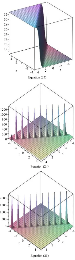
So that the exact solution of Equation (14)

Case 1.

when

λ

2−4

µ

>0,

µ

≠0,

(

)

(

)

2 2 1 2 2 1 3 3 2 ₄ 4 tanh 2 3 3 2 ₄ 4 tanh 2 u u C C µλ µ λ µ

λ µ ξ λ

µλ µ

λ µ

λ µ ξ λ

− = −  ₋    − − + −     − = −  ₋    − − _ + _−   (23)

when

λ

2−4

µ

>0,

µ

=0,

(

)

(

)

(

)

(

)

2 2 1 1

3 3 3

,

2 2 exp 1 2 exp 1

u C C λ λ µ λ ξ λ ξ   − = − − _ _ + −

+ − _ _ (24)

when

λ

2−4

µ

=0,

µ

≠0,

λ

≠0,

(

)

(

)

(

)

(

)

2 1 1 2 1 1

3 2 2 2

3 3 ) , 2 2 C C u C C

λ ξ λ ξ

µ

λ ξ λ ξ

 

+ + + +

−

= + − _ _

+ _ + _ (25)

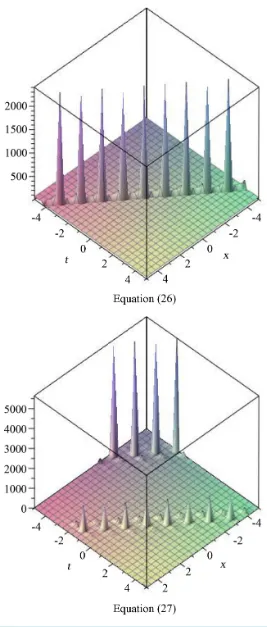
when

λ

2−4

µ

=0,

µ

=0,

λ

=0,

(

)

2

1 1

3 3 3 1

,

2 2 2

u C C λ µ ξ ξ   − = − _{− } _

+ _ + _ (26)

(5)

(

)

(

)

2 2 1 2 2 2 1 3 3 2 ₄ 4 tan 2 3 2 , 2 ₄ 4 tan 2 u C C µλ µ µ λ

µ λ ξ λ

µ µ λ

µ λ ξ λ

− = −  ₋    − + −           −      −    − + −  _ _   _ _    (27) Case 2.

when

λ

2−4

µ

>0,

µ

≠0,

(

)

(

)

2 2 2 1 2 2 2 1

1 1 3

2 4 ₄

4 tanh 2 3 2 2 ₄ 4 tanh 2 u C C µλ µ λ λ µ

λ µ ξ λ

µ

λ µ

λ µ ξ λ

− = − −  ₋    − − + −           −      _ − _  − − + −  _ _   _ _    (28)

when

λ

2−4

µ

>0,

µ

=0,

(

)

(

)

(

)

(

)

2 2 2 1 1

1 1 3 3

,

2 4 2 exp 1 2 exp 1

u C C λ λ µ λ λ ξ λ ξ   − = − − − _ _ + −

+ − _ _ (29)

when

λ

2−4

µ

=0,

µ

≠0,

λ

≠0,

(

)

(

)

(

)

(

)

(

)

(

)

2 1 1 2 2 1 1

3 2 2 2

1 1 3

,

2 4 2

C C

u

C C

λ ξ λ ξ

µ λ

λ ξ λ ξ

 

+ + + +

−

= − + − _ _

+ _ + _ (30)

when

λ

2−4

µ

=0,

µ

=0,

λ

=0,

(

)

2 2

1 1

1 1 3 3 1

,

2 4 2 2

u C C λ µ λ ξ ξ   − = − − ₊ _{− } ₊ 

  (31) when

λ

2−4

µ

<0,

(

)

(

)

2 2 2 1 2 2 2 1

1 1 3

2 4 ₄

4 tan 2 3 2 , 2 ₄ 4 tan 2 u C C µλ µ λ µ λ

µ λ ξ λ

µ µ λ

µ λ ξ λ

− = − −  ₋    − + −           −      −    − + −  _ _   _ _    (32)

3.2. Example 2: The (3+1)-Dimensional KP Equation

(6)

2

6 6 0.

xt x xx xxxx yy zz

u + u + uu −u −u −u = (33)

Xie et al. [35] obtained non-traveling wave solutions by the improved tanh function method, in which they introduced a generalized Riccati equation and gained its 27 new solutions. In this paper, we will construct new non-traveling wave solution of Equation (33). As a result, new non-traveling wave solutions including soliton- like solutions and periodic solutions of Equation (1) are obtained. A generalized variable-coefficient algebraic method with computerized symbolic computation is developed to deal with (3+1)-dimensional KP equation with variable coefficients in [36]. Chen et al. [37] study (3+1)-dimensional KP equation by using the new generalized transformation in homogeneous balance method.

Using the wave variable ξ = + + −x y z ct, the Equation (33) is carried to an ODE of the form

(

)

( )

2

2 6 6 0.

c u′′ u′ uu′′ u′′′

− + + + − = (34)

Integrating twice and setting the constants of integration to zero, we obtain

(

)

2

2 3 0.

c u u u′′

− + + − = (35)

Balancing u′′ and u2 in Equation (35) yields, m+ =2 2m⇒ =m 2. Consequently, we get the formal solution (15).

Substituting (15)-(17) into Equation (35) and equating the coefficients of exp

(

−4ϕ ξ

( )

)

, exp

(

−3ϕ ξ

( )

)

,

( )

(

)

exp −2ϕ ξ , exp

(

−ϕ ξ

( )

)

, exp

(

−0ϕ ξ

( )

)

to zero, we respectively obtain

2

2 2

3a −6a =0, (36)

1 2 1 2

6a a −2a −10a λ=0, (37)

(

)

2 2

2 0 2 1 1 2 2

2 6 3 3 8 4 0,

c a a a a a

λ

a

µ

a

λ

− + + + − − − = (38)

(

)

2

1 0 1 1 1 2

2 6 2 6 0,

c a a a a

µ

a

λ

a

λµ

− + + − − − = (39)

(

)

5 2

0 0 1 2

2 3 2 0.

c a a a

λµ

a

µ

− + + − − = (40)

From Equations (36)-(40), we have the following results:

Case 1.

2

0 1 2

2 4 , 2 , 2 , 2.

c= − +

µ λ

− a =

µ

a =

λ

a =

Case 2.

2 2

0 1 2

2 1

4 2, , 2 , 2.

3 3

c= − µ λ+ − a = µ+ λ a = λ a =

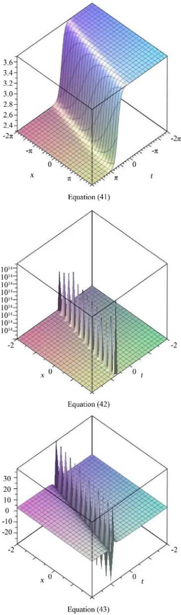
So that the exact solution of equation

Case 1.

when

λ

2−4

µ

>0,

µ

≠0,

(

)

(

)

2 2 1 2 2 2 1 4 2 4 4 tanh 2 2 2 , 4 4 tanh 2 u C C µλ µ λ µ

λ µ ξ λ

µ

λ µ

λ µ ξ λ

= +  ₋    − − _ + _−         +     ₋ ₋ _ − ₊ _₋   _ _   _ _    (41)

when

λ

2−4

µ

>0,

µ

=0,

(

)

(

)

(

)

2 2 1 1 2

2 2 ,

exp 1 exp 1

u

C C

λ λ

µ

λ ξ λ ξ

 

= + + _ _

(7)

when

λ

2−4

µ

=0,

µ

≠0,

λ

≠0,

(

)

(

)

(

)

(

)

2 1 1 2 1 1

4 2 2 2

2 C 2 C ,

u

C C

λ ξ λ ξ

µ

λ ξ λ ξ

 

+ + + +

= − + _ _

+ _ + _ (43)

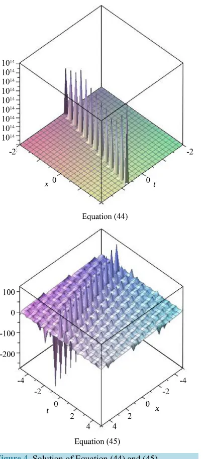
when

λ

2−4

µ

=0,

µ

=0,

λ

=0,

2

1 1

2 1

2 2 ,

u C C λ µ ξ ξ   = + _{+ } _

+ _ + _ (44)

when

λ

2−4

µ

<0,

(

)

(

)

2 2 2 2 2 1 1 4 2

2 2 ,

4 4

4 tan 4 tan

2 2

u

C C

µλ µ

µ

µ λ µ λ

µ λ ξ λ µ λ ξ λ

      = + +    ₋    ₋       − _ + _− _ − _ + _− _       (45) Case 2.

when

λ

2−4

µ

>0,

µ

≠0,

(

)

(

)

2 2 2 2 2 2 1 1

2 1 4 2

2 ,

3 3 ₄ ₄

4 tanh 4 tanh

2 2

u

C C

µλ µ

µ λ

λ µ λ µ

λ µ ξ λ λ µ ξ λ

      = + + +    −    −       − − _ + _− _− − _ + _− _       (46)

when

λ

2−4

µ

>0,

µ

=0,

(

)

(

)

(

)

2 2 2 1 1

2 1 2

2 ,

3 3 exp 1 exp 1

u

C C

λ λ

µ λ

λ ξ λ ξ

 

= + + + _ _

+ − _ + − _ (47)

when

λ

2−4

µ

=0,

µ

≠0,

λ

≠0,

(

)

(

)

(

)

(

)

2 1 1 2 2 1 1

4 2 2 2

2 1 2 , 3 3 C C u C C

λ ξ λ ξ

µ λ

λ ξ λ ξ

 

+ + + +

= + − + _ _

+ _ + _ (48)

when

λ

2−4

µ

=0,

µ

=0,

λ

=0,

2 2

1 1

2 1 2 1

2 , 3 3 u C C λ µ λ ξ ξ   = + + _{+ } _

+ _ + _ (49)

when

λ

2−4

µ

<0,

(

)

(

)

2 2 2 2 2 2 1 1

2 1 4 2

2 ,

3 3 ₄ ₄

4 tan 4 tan

2 2

u

C C

µλ µ

µ λ

µ λ µ λ

µ λ ξ λ µ λ ξ λ

      = + + +    ₋    ₋       − _ + _− _ − _ + _− _       (50)

4. Conclusion

(8)

[image:8.595.236.396.157.707.2]

equation and (3+1)-dimensional Kadomstev-Petviash-vili which have been constructed using the modified simple equation method. Let us compare between our results obtained in the present article with the well-known results obtained by other authors using different methods as follows: Our results of (2+1)-dimensional soliton breaking equation and (3+1)-dimensional Kadomstev-Petviash-viliare are new and different from those obtained in [38][39]. Figures 1-4 show the solitary wave solutions of equations. It can be concluded that this method is

(9)

[image:9.595.180.447.83.710.2]

(10)

[image:10.595.222.404.86.703.2]

(11)

[image:11.595.216.418.84.541.2]

Figure 4. Solution of Equation (44) and (45).

reliable and propose a variety of exact solutions NPDEs. The performance of this method is effective and can be applied to many other nonlinear evolution equations.

References

[1] Ablowitz, M.J. and Segur, H. (1981) Solitions and Inverse Scattering Transform. SIAM, Philadelphia. http://dx.doi.org/10.1137/1.9781611970883

[2] Malfliet, W. (1992) Solitary Wave Solutions of Nonlinear Wave Equation. American Journal of Physics, 60, 650-654. http://dx.doi.org/10.1119/1.17120

[3] Malfliet, W. and Hereman, W. (1996) The Tanh Method: Exact Solutions of Nonlinear Evolution and Wave Equations.

Physica Scripta, 54, 563-568. http://dx.doi.org/10.1088/0031-8949/54/6/003

[4] Wazwaz, A.M. (2004) The Tanh Method for Travelling Wave Solutions of Nonlinear Equations. Applied Mathematics and Computation, 154, 714-723. http://dx.doi.org/10.1016/S0096-3003(03)00745-8

(12)

Liouville Equation Arising in Mathematical Physics and Biology. International Journal of Computer Applications,

112.

[6] Zahran, E.H.M. and Khater, M.M.A. (2014) Exact Traveling Wave Solutions for the System of Shallow Water Wave Equations and Modified Liouville Equation Using Extended Jacobian Elliptic Function Expansion Method. American Journal of Computational Mathematics, 4.

[7] Zahran, E.H.M. and Khater, M.M.A. (2014) The Modified Simple Equation Method and Its Applications for Solving Some Nonlinear Evolutions Equations in Mathematical Physics. Jökull Journal, 64.

[8] Khater, M.M.A. (2015) The Modified Simple Equation Method and Its Applications in Mathematical Physics and Bi-ology. Global Journal of Science Frontier Research: F Mathematics and Decision Sciences, 15.

[9] Wazwaz, A.M. (2004) A Sine-Cosine Method for Handling Nonlinear Wave Equations. Mathematical and Computer Modelling, 40, 499-508. http://dx.doi.org/10.1016/j.mcm.2003.12.010

[10] Yan, C. (1996) A Simple Transformation for Nonlinear Waves. Physics Letters A, 224, 77-84. http://dx.doi.org/10.1016/S0375-9601(96)00770-0

[11] Fan, E. and Zhang, H. (1998) A Note on the Homogeneous Balance Method. Physics Letters A, 246, 403-406. http://dx.doi.org/10.1016/S0375-9601(98)00547-7

[12] Wang, M.L. (1996) Exct Solutions for a Compound KdV-Burgers Equation. Physics Letters A, 213, 279-287. http://dx.doi.org/10.1016/0375-9601(96)00103-X

[13] Abdou, M.A. (2007) The Extended F-Expansion Method and Its Application for a Class of Nonlinear Evolution Equa-tions. Chaos, Solitons & Fractals, 31, 95-104. http://dx.doi.org/10.1016/j.chaos.2005.09.030

[14] Ren, Y.J. and Zhang, H.Q. (2006) A Generalized F-Expansion Method to Find Abundant Families of Jacobi Elliptic Function Solutions of the (2+1)-Dimensional Nizhnik-Novikov-Veselov Equation. Chaos, Solitons & Fractals, 27, 959-979. http://dx.doi.org/10.1016/j.chaos.2005.04.063

[15] Zhang, J.L., Wang, M.L., Wang, Y.M. and Fang, Z.D. (2006) The Improved F-Expansion Method and Its Applications.

Physics Letters A, 350, 103-109. http://dx.doi.org/10.1016/j.physleta.2005.10.099

[16] He, J.H. and Wu, X.H. (2006) Exp-Function Method for Nonlinear Wave Equations. Chaos, Solitons & Fractals, 30, 700-708. http://dx.doi.org/10.1016/j.chaos.2006.03.020

[17] Aminikhad, H., Moosaei, H. and Hajipour, M. (2009) Exact Solutions for Nonlinear Partial Differential Equations via Exp-Function Method. Numerical Methods for Partial Differential Equations, 26, 1427-1433.

[18] Zhang, Z.Y. (2008) New Exact Traveling Wave Solutions for the Nonlinear Klein-Gordon Equation. Turkish Journal of Physics, 32, 235-240.

[19] Abdelrahman, M.A.E., Zahran, E.H.M. and Khater, M.M.A. (2015) Exact Traveling Wave Solutions for Modified Liouville Equation Arising in Mathematical Physics and Biology. International Journal of Computer Applications,

112.

[20] Zahran, E.H.M. and Khater, M.M.A. (2015) The Two-Variable G

G

′      ,

1

G

   

 -Expansion Method for Solving Nonlinear Dynamics of Microtubles—A New Model. Global Journal of Science Frontier Research: A Physics and Space Science,

15, Version 1.0.

[21] Zayed, E.M.E. and Gepreel, K.A. (2009) The G

G

′    

 -Expansion Method for Finding Traveling Wave Solutions of Nonlinear Partial Differential Equations in Mathematical Physics. Journal of Mathematical Physics, 50, Article ID: 013502. http://dx.doi.org/10.1063/1.3033750

[22] Zahran, E.H.M. and Khater, M.M.A. (2014) Exact Solutions to Some Nonlinear Evolution Equations by Using G

G

′      - Expansion Method. Jökull Journal, 64.

[23] Dai, C.Q. and Zhang, J.F. (2006) Jacobian Elliptic Function Method for Nonlinear Differential Difference Equations.

Chaos, Solitons & Fractals, 27, 1042-1049. http://dx.doi.org/10.1016/j.chaos.2005.04.071

[24] Fan, E. and Zhang, J. (2002) Applications of the Jacobi Elliptic Function Method to Special-Type Nonlinear Equations.

Physics Letters A, 305, 383-392. http://dx.doi.org/10.1016/S0375-9601(02)01516-5

[25] Zahran, E.H.M. and Khater, M.M.A. (2014) Exact Traveling Wave Solutions for the System of Shallow Water Wave Equations and Modified Liouville Equation Using Extended Jacobian Elliptic Function Expansion Method. American Journal of Computational Mathematics, 4, 455-463. http://dx.doi.org/10.4236/ajcm.2014.45038

(13)

Construct New Double-Periodic Solutions for the Generalized Ito System. Chaos, Solitons & Fractals, 28, 112-126. http://dx.doi.org/10.1016/j.chaos.2005.05.016

[27] Abdelrahman, M.A.E., Zahran, E.H.M. and Khater, M.M.A. (2014) Exact Traveling Wave Solutions for Power Law and Kerr Law Non Linearity Using the exp

(

−ϕ ξ

( )

)

-Expansion Method. The Global Journal of Science Frontier Re-search (GJSFR), 14, Version 1.0.

[28] Abdelrahman, M.A.E. and Khater, M.M.A. (2015) The Exp

(

−ϕ ξ

( )

)

Expansion Method and Its Application for Solving Nonlinear Evolution Equations. International Journal of Science and Research (IJSR), 4, 2143-2146.

[29] Abdelrahman, M.A.E., Zahran, E.H.M. and Khater, M.M.A. (2015) The exp

(

−ϕ ξ

( )

)

-Expansion Method and Its Ap-plication for Solving Nonlinear Evolution Equations. International Journal of Modern Nonlinear Theory and Applica-tion, 4, 37-47. http://dx.doi.org/10.4236/ijmnta.2015.41004

[30] Hirota, R. and Ohta, Y. (1991) Hierarchies of Coupled Soliton Equations I. Journal of the Physical Society of Japan,

60, 798-809. http://dx.doi.org/10.1143/JPSJ.60.798

[31] Zhang, S. (2007) New Exact Non-Traveling Wave and Coefficient Function Solutions of the (2+1)-Dimensional Breaking Soliton Equations. Physics Letters A, 368, 470-475. http://dx.doi.org/10.1016/j.physleta.2007.04.038

[32] Cheng, Y. and Li, B. (2003) Symbolic Computation and Construction of Soliton-Like Solutions to the (2+1)-Dimen- sional Breaking Soliton Equation. Communications in Theoretical Physics, 40, 137-142.

http://dx.doi.org/10.1088/0253-6102/40/2/137

[33] Peng, Y.Z. (2005) New Exact Solutions for (2+1)-Dimensional Breaking Soliton Equation. Communications in Theo-retical Physics, 43, 205-207. http://dx.doi.org/10.1088/0253-6102/43/2/004

[34] Peng, Y.Z. and Krishna, E.V. (2005) Two Classes of New Exact Solutions to (2+1)-Dimensional Breaking Soliton Eq-uation. Communications in Theoretical Physics, 44, 807-809. http://dx.doi.org/10.1088/6102/44/5/807

[35] Xie, F.D., Zhang, Y. and Lu, Z.S. (2005) Symbolic Computation in Non-Linear Evolution Equation: Application to (3+1)-Dimensional Kadomtsev-Petviashvili Equation. Chaos, Solitons & Fractals, 24, 257-263.

http://dx.doi.org/10.1016/S0960-0779(04)00552-1

[36] Zhao, H. and Bai, C. (2006) New Doubly Periodic and Multiple Soliton Solutions of the Generalized (3+1)-Dimen- sional Kadomtsev-Petviashvilli Equation with Variable Coefficients. Chaos, Solitons & Fractals, 30, 217-226. http://dx.doi.org/10.1016/j.chaos.2005.08.148

[37] Chen, Y., Yan, Z. and Zhang, H. (2003) New Explicit Solitary Wave Solutions for (2+1)-Dimensional Boussinesq Eq-uation and (3+1)-Dimensional KP EqEq-uation. Physics Letters A, 307, 107-113.

http://dx.doi.org/10.1016/S0375-9601(02)01668-7

[38] Bekir, A. and Uygun, F. (2012) Exact Traveling Wave Solutions of Nonlinear Evolution Equations by Using the G

G

′

-Expansion Method. Arab Journal of Mathematical Sciences, 18, 73-85. http://dx.doi.org/10.1016/j.ajmsc.2011.08.002 [39] Zahran, E.H.M. and Khater, M.M.A. (2014) The Modified Simple Equation Method and Its Applications for Solving