Munich Personal RePEc Archive
Active Labour Market Policies and
Unemployment Convergence in
Transition
Tyrowicz, Joanna and Wójcik, Piotr
University of Warsaw
2009
Online at
https://mpra.ub.uni-muenchen.de/15201/
Active Labour Market Policies and Unemployment
Convergence in Transition
∗
Joanna Tyrowicz
† University of WarsawPiotr W´
ojcik
University of Warsaw
First version: February, 2007
This version: March, 2009
Abstract
In this paper we approach the issue of social cohesion across NUTS4 regions in Poland. We analyse regional dynamics of unemployment rates and try to evaluate the impact of Active Labour Market Policies (ALMPs) in observed trends. Using data for 1999 till 2008 we employ tools typically applied to income convergence analyses to test the stability of unemployment distribution - both unconditionally and taking into account explanatory power of unemployment structure and ALMPs in Polish regions. Our findings suggest no unconditional convergence understood both in terms of levels and in terms of dispersion, while the latter seems to suggest ”convergence of clubs” within a group highest unemploy-ment regions. The analysis comprised as well accounting for potential impact of ALMPs, controlling for differentiated unemployment structure. We find no evidence that cohesion efforts contribute to the convergence or less of the divergence phenomena.
Key words: regional unemployment rate differentials, convergence analysis, Poland
JEL Codes: J43, R23, R58, E64, J18
1
Introduction
Poland belongs to the highest unemployment rate group among European Union Member States. Financ-ing of active labour market policies has been intensified gradually as of 2004, reachFinanc-ing over 0.2% of GDP in 2006. Nonetheless, these policies covered barely 20% of the unemployed, with some evidence of “cream-ing”, (Tyrowicz 2006). Consequently, despite general decrease in national unemployment, some regions still struggle with 40% unemployment rate thresholds. Thus inquiring regional structural dynamics of unemployment seems necessary to understand the mechanics of labour market movements in Poland.
Some researchers suggest that approximately 80% of unemployment can be characterised as structural,
(Sztanderska and Socha 2001), but these results address both frictional andstricte structural
unemploy-ment, while geographical issues are not explored. Comparing these estimates to a share of unemployed still entitled to unemployment benefit (approximately 75% to 87% throughout the analysed period) pro-vides additional grounds to this statement. The aim of this paper is to inquire the (time) stability of the (geographical) distribution pattern, assessing additionally to what extent the interplay of active labour market policies (ALMPs) and economic outlook have influenced the local labour market developments.
The situation in the labour market in Poland has been extremely difficult for the past years, with the unemployment rates consistently above 16-18% thresholds (Polish Labour Force Survey, 2006), while the
∗Authors are grateful for very valuable comments to Badi Baltagi, Roger Bivand and Ryszard Kokoszczynski, Michal
Alexeev, participants of various seminars at Paris I - Sorbonne, Indiana University and the University of Warsaw as well as NEM 2007 in Tallinn, CAPE 2007 in Nuremberg and XXII AIEL in Naples and MET-EACES in London conferences. We are also indebted to two anonymous referees. The remaining errors are, of course, ours. Part of the work has been performed while Joanna Tyrowicz was a Visiting Researcher at IZA in Bonn, whose support is gratefully acknowledged.
odds to become long-term unemployed exceed 50%. At the same time, as noted by Munich, Svejnar and Terrel (1998), Poland had one of the lowest among the Central and Eastern European Countries (CEECs) outflow rates. Vacancies ratios are dramatically low throughout the whole transition period, with averages
around a thousand job-seekers per one offer1. Reported unemployment exhibits that approximately 700
000 of young women has no or negligible work experience, with gender employment gap among young and 50+ women doubling the EU average. At the same time labour activity in the group 50+ is among the lowest in the whole EU (at 26%).
There are at least two main motivations to inquire the dynamics of local labour markets. First, most macro-level models assume implicitly homogeneity and symmetry of shock response at least within countries. This assumption is not always rooted in data. In the case of EU for example, studies find income convergence between nations and divergence on more disaggregated levels, both within and across countries (for example, Egger and Pfaffermayr (2005) or Paas and Schlitte (2007)). This problem seems
to receive more attention in the recent years2. The second reason is more rooted in the policy choice
area. Within Europe, cohesion and catching up of the regions lagging behind are not only one of the main policy objectives but also a constituent expression of Community values. These values are frequently transferred to national levels, where cohesion, equal access and convergence receive attention both explicitly in constitutions and laws and implicitly in financing algorithms. For example, in Poland any labour market policies financing is distributed with preference to areas with (i) higher than average unemployment rate, (ii) higher than average share of long-term unemployed and (iii) higher than average number of unemployed. Consequently, regions facing relative hardships receive more resources to alleviate their impact.
In this paper we apply β- andσ-convergence analyses to the registered unemployment data covering
the period 1999-2008. We use a unique data on active labour market policies and unemployment structure, which have not been analysed before. The technique of kernel density estimates for convergence analysis
is applied to unemployment rates on NUTS4 (poviat). The period we chose captures the so-called ”second
wave of unemployment” commencing in 2001 as well as implementing ALMPs on a more comprehensive scale (from less than 10% up to 25% of unemployed subjected to active instruments). Taking into account the emphasised structural character of Polish unemployment as well as challenges this situation implies, we employed a technique typically applied to income analysis allowing to inquire, whether any regional differences in development patterns may be observed. Notably, we test the hypotheses of convergence of levels as well as the stability of unemployment rates distribution. The first of the questions is approached with the use of econometrics, whereas the latter is addressed with the use of nonparametric kernel density estimates3.
This paper is organised as follows. We briefly discuss the literature, subsequently proceeding to de-scribing the methodology in section 3. Section 4 covers data. Section 5 presents the main findings with
reference to distribution dynamics, while section 6 focuses on main findings of β-convergence analysis.
Section 7 concludes.
2
Literature review
In Poland, the process of employment restructuring consisted mainly of the reductions in employment with growing average job tenure as well as average time spent in unemployment or inactivity (Svejnar 2002a).
1
The principal studies in this area are carefully surveyed in M¨unich, Svejnar and Terrell (1997).
2
For example, Armstrong and Taylor (2000) argue that one should focus on the problem of adjustment speed as well as persistence of potential unemployment differentials, instead of aggregate convergence per se, since some effects may accumulate over time, effectively altering the direction of adjustments. Further on the theoretical grounds, Boeri and Terrell (2002) inquire whether these differentials could be explained on the grounds of optimal transition speed theory (Ferragina and Pastore (2008) provide an extensive review of this issue).
3
Dismissals - if compensated at all - found their outcome with hiring of young, better educated workers, but the youth unemployment rate for a long time continued to be the highest in Europe as well as by age groups in Poland. People who lost their employment usually became permanently unemployed or inactive
(Grotkowska 2006) with currently less than 13% of the unemployed still retaining the right to benefit4,
thus suggesting that most of the unemployed are either long-term unemployed or have a long record of unstable, short-term employment.
Consequently, on an individual level it is usually easy to identify the ideal type of winners and losers in the transition process. However, in terms of regional analysis the ”conventional wisdom” of Eastern Poland generally lagging behind finds no support in data, while some of the highest unemployment regions are located relatively close to the ”growth poles”, (Gorzelak 1996), which stays in contrast to the categori-sation suggested by the literature before. Unemployment convergence at regional level received recently considerable attention from the academics. Buettner (2007) compares empirical evidence on regional labor market flexibility in Europe. Marelli (2004) as well as Huber (2007) provide an overview of similarities and disparities across European Union regions. In particular, it seems that CEE countries exhibit higher regional wage flexibility, (Buettner 2007). At the same time, despite phenomenal migrations emerging af-ter 2004, labour mobility is still assessed to be low (Kaczmarczyk and Tyrowicz 2008), while Fihel (2004) demonstrates that effectively in the local scale unemployment is not significant as pushing factor (these issues have been surveyed, among others, by Huber (2007)). For the case of CEECs, the role of transition processes may indeed still be significant (Svejnar 2002b).
Using earlier data, Scarpetta and Huber (1995) construct a measure that captures both the degree of economic development and the structure of industry in a single index - economic development is proxied
by an index of industrial diversification, where regions are classified to six groups5. In a similar vein, G´ora
and Lehman (1995) classify voivodships by the degree of economic development of a region, but build
on employment shares of services and industry in 1990, relative change in total employment and that of employment in services and the relative per capita income of municipalities in 1992. In addition, Lehmann
and Walsh (1998) build an economic classification ofvoivodships with an intention to produce an index
reflecting the degree of employment restructuring with the use of seven indicators: share of services in employment; share of short-tenured men (i.e. with tenure less than ten years) in total male employment;
number of telephonesper capita;voivodship shares of domestic and direct foreign investment, normalised
on population; share of construction in total employment and share of agriculture in total employment.
However, although these indices correlate reasonably well among each other, correlation with voivodship
unemployment rates is highly unsatisfactory (Newell and Pastore 1999). Moreover, these findings no longer hold if one disaggregated to NUTS4 level (units with on average over 6 000 unemployed in the labour market distress period and over 40 000 in the labour force).
Taking a different perspective, Newell and Pastore (1999) argue that it is the hazard of job loss differentiating for employees with longer tenure that drives the regional differences, but these findings cover 1995-1999 time span (a period of gradual improvement in both economic and labour market outlooks) and are no longer consistent with more recent (2001-2005) developments (Grotkowska 2006), namely, explanatory power of these hazard differentials disappears with the general growth of unemployment
4
In Poland the entitlement to unemployment benefit is temporary and lasts only 12 months after the registration (18 months in regions with more labour market hardships). After this period, unemployment benefits may be replaced by social assistance (which is lower and bases on family income and not labour market status). The entitlement to unemployment benefit is re-established for an unemployed who obtains legal employment for a period above 6 months. No publicly available statistics report the effective share of long-term unemployed or unemployment duration. For example, if one does not confirm ”willingness to undertake employment”, one is de-listed from the unemployment registries. However, 3 months after this occurrence, one may register again (the basic incentive is free access to public health care system for the unemployed and his/her family) and then, the unemployment tenure is calculated from the scratch. However, benefit entitlements are not. Consequently, the share of unemployed still retaining the right to the benefit is a reliable measure of actual rate of long-term unemployment.
5
rate. Thus, the persistence of high unemployment rate regional differentials remains as intriguing as the persistence of high unemployment itself.
In the empirical literature of unemployment rate characteristics, one can find a number of
differen-tiated approaches towards the unemployment rate dynamics and persistence as well as distribution (cfr.
Decressin and Fatas (1995), Obstfeld and Peri (1998) or more recently Armstrong and Taylor (2000)). Perugini, Polinori and Signorelli (2005) use NUTS2 level data and inquire the regional differentiation of Poland and Italy. Marelli (2004) focuses on specialisation for NUTS2 EU regions with tripartite desaggre-gation (industrial, agricultural and service sectors) reaching the conclusion that convergence in economic structures occurs, while income does not. However, Marelli (2004) analyses predominantly income and economic convergence and not explicitly the underlying fundamentals (like, for example, labour markets performance). Overman and Puga (2002) perform conditional kernel density analyses of European un-employment rates taking into account the distributions of underlying fundamentals (eg. the skills, the regional specialisation as well as the growth rates of population and the labour force).
Suggesting a different angle, Bayer and Juessen (2006) perform a unit-root test on regional unem-ployment rate differentials using Mikrozensus data for West Germany over the 1960-2002 time span. By differentiating between the theoretically motivated imperative of convergence itself (Blanchard and Katz 1992) and the speed of adjustment (as argued by Armstrong and Taylor (2000)) they focus on the concept of stochastic convergence (Carlino and Mills 1993). In this framework, convergence is present only if shocks to the unemployment differential are temporary, thus erasing disparities between regions, providing a testable hypothesis of regional and national unemployment rates cointegration. Bayer and Juessen (2006) find moderate evidence in support of the convergence hypothesis. Similar technique has been applied by Gomes and da Silva (2006) for the regions of Brazil finding strong evidence of hysteresis and unemployment regional differential persistence.
However, one can put forward a strong argument against these results, namely that stationarity of the regional unemployment rates differentials can happen both under convergence and divergence scenarios, let alone trend stationarity. Notably, with some regularity in the cycles, unemployment rate differentials can positively pass the unit-root test even if real differentials are growing (some regions still suffering harder during the crisis and recovering less with the good economic outlooks). Thus, in this paper a different approach is followed, namely we analyse the conditional density functions with kernel estimates, assessing the changes in each region’s position in the nation-wide unemployment rate distribution. Bianchi and Zoega (1999) use non-parametric kernel density methods to test the hypothesis of multimodality in regional unemployment rates distribution across counties of the UK, thus analysing the patterns of variance. They found that regional transition probabilities are similar for both high and low unemployment counties with the persistence of 97%.
3
Methodology
Empirical strategy for verifying the convergence hypothesis developed so far are varied. The most obvious
is the test ofβconvergence (unconditional and conditional). Findingβconvergence corresponds to proving
that levels of unemployment converge to a common rate, while levels themselves may be conditioned on
structural parameters characterising particular local labour market. Consequently, unconditionalβ
con-vergence describes one common level for all regions, whereas conditional one allows for differentiated levels
for groups of structurally similar communities. One can also inquire if the dispersion of unemployment
lowers over time and this may be approached testing forσconvergence. Finally, one can try to investigate
how persistent the regional unemployment rate differentials are, by applying the concept of stochastic
convergence6. Importantly,β-convergence is a necessary, but not a sufficient condition of σ-convergence.
In principle, in the case of conditional β-convergence one could expect that within the groups of units
approaching the samelevel, also dispersion around it lowers leading toσtype convergence of clubs.
6
The most appropriate tool to approachσtype convergence is provided by kernel density estimates. In general, they approximate an unknown density function for a random variable, basing on a finite number of observations drawn from this distribution. This estimator is continuous equivalent of the histogram. The values of the density function at some point are calculated as relative frequency of the observations in the nearest surrounding of this point (bandwidth window), while this relative frequency is estimated using a density function (kernel).
Although the choice of the kernel function has evident but in fact only slight impact on the way the unknown density functions are estimated, it is the bandwidth window that essentially drives the results. The imposed size predetermines the degree of the curve or surface smoothening. Too wide bandwidth window will hide the real data distribution, while too narrow might misleadingly result in function with multiple vertices - not necessarily true in reality and rather troublesome in terms of interpretation. Sil-verman (1986) provides the procedures for finding optimal bandwidth, subject to differentiated kernel functions, basing on standard deviations and inter-quartile differentials (independently for all vectors in the case of multidimensional distributions). An extension of this approach is to use adaptive kernel den-sity estimation, which allows for differentiated bandwidths for each observation and this is the method we employ in the paper.
If the initial unemployment rate is defined by x, while the one for the current period by x+ 1, the
distribution ofx+ 1 conditional on xmay be written down as:
f[x+ 1|x] = f[x, x+ 1] fx[x]
, (1)
wherefx[x] is the marginal distribution of the initial unemployment rate, whilef[x, x+ 1] represents the
combined distribution of xandx+ 1. Estimating the conditional density function, both numerator and
denominator of (1) are replaced by non-parametric estimators. By stating that adaptive kernel estimation is employed to estimate marginal distribution of the initial unemployment rates we mean specifically that one-dimensional distributions are applied, i.e.:
ˆ fA
x[x] = 1 n N X i=1 1 hxwi
Kx−xi hxwi
, (2)
wherenis the number of observations,hxis the bandwidth window for the initial unemployment rate and
K[.] represents the kernel function7. At the first stage, weightsw
i take the value of 1 for all observations.
The combined distribution of initial and final unemployment distribution i.e. the denominator of equation (1), is thus estimated by:
ˆ fA
xt,xt+1[x] =
1 n N X i=1 1 hxhx+1wi2
Kx−(x+ 1)i hxwi
K
(x+ 1)−(x+ 1)i
hx+1wi
, (3)
where hx+1 is the bandwidth window for the final unemployment rate distribution, while subscript A
signifies the use of adaptive technique.
Importantly, at the first stage combined density function is estimated with the optimal bandwidth window, while weights are uniform for all observations. Subsequently, basing on these estimates, local differentiation of bandwidth windows are calculated according to:
wi=
1 n N X i=1 1 hxhx+1wi2
K
x−xi
hxwi
K
(
x+ 1)−(x+ 1)i
hx+1wi
1/2
. (4)
In this expression, the denominator of the formula in the parentheses is the combined density function
estimator calculated with the use of uniform weights and bandwidth window8, while the numerator gives
7
With the large number of observations (over 400 units for Poland) we uniformly used the Gaussian kernel function, thus implicitly assuming normal distribution. However, Gaussian assumption is by far the most frequently used one, while it only concerns the properties of the nearest surrounding of each point (within the bandwidth windows) and not the distribution as a whole.
8
the geometric average of this estimator for matching couples of both variables. The final conditional density function is found basing on the weights from equation (4) to equations (2) and (3) (calculating
their quotient), according to equation (1)9.
This methodology has shorthand interpretative advantages. First of all, convergence/divergence may be easily detected from the graphs of the conditional density functions. Namely, vertical shape of this function suggests divergence, while horizontal alignment is consistent with the convergence hypothesis.
If the conditional density function follows the 45◦ line, overall density function exhibits stability, i.e. an
observation drawn randomly at one point in time is highly unlikely to move towards relatively higher or lower values in any preceding or subsequent point in time. Stability implies directly that neither divergence nor convergence of distribution can be tracked.
The conditional distribution is obtained by regressing growth rates of the unemployment rate on a distributed lags of the single conditioning variable and extracting the residuals for subsequent analysis. The residuals from the regression contain the part of the growth rate of unemployment that is not explained by the analyzed factor. Prior to the analysis we conduct Granger causality tests, to take into account only these variables that seem to have impact on unemployment rate dynamics, at the very least in the sense of being leading indicators of subsequent changes.
Finally, these residual growth rates are used to calculate the distribution of unemployment rates with the impact of the analyzed variable. In our causality analysis we assume a horizon of half a year - taking six lags of the growth rate of the independent variable to explain the regional unemployment growth rate. The method derives from that suggested by Sims (1972) and implemented subsequently by Quah (1996). Consequently, we implicitly assume one directional causality of analyzed factor at the unemployment rate. While not in all cases this would be justified, the main concern of this paper concerns dynamics of the unemployment rate distributions. Therefore, even if some reverse causality was in play, the analysed direction would still be active, whilst kernel density analysis is non-parametric and hence not susceptible to eventual inconsistency issues.
4
Data
In the paper monthly data covering the period from January 1999 till June 2008 were used at the lowest
available administration level ofpoviats (NUTS4). This paper uses for the first time unique
administra-tive data on unemployment structure (as of January 2000) and ALMPs spendings (as of January 2001) reported consistently by labour offices at NUTS4 level. We treat structure variables as control factors while financing of active labour market policies plays the role of proxy for policy measures. We construct three measures: spendings per person in any treatment by public employment services, spendings per unemployed (irrespectively of whether he/she was in treatment or not) and share of unemployed in any
treatment offered by public employment services, i.e. coverage. These measures were meant to capture
intensity, depth and extensiveness of active labour market policies use, respectively10.
Using more aggregate level would diminish the value added of the analysis in at least two ways. First
of all, NUTS2 level (Polishvoivodships) do not perform any active labour market policies, which implies
that outcomes are not dependent upon efforts made at this level, but rather aggregate of different (approx-imately 20-30) lower level administrative units. Secondly, NUTS2 units are relatively large and therefore less diversified both when it comes to comparing unemployment levels and unemployment structure. In-deed, NUTS2 units are so big and heterogeneous that only slight differentiation of unemployment rates may be observed (lowest to highest ratio amounts to only 1:1.5 at NUTS2 and as much as 1:25 at NUTS4). Due to the administrative changes in Poland in 1999 no data before that moment are available at NUTS4 level. At the same time, this period covers the so-called “second wave of unemployment”, commencing with the economic slowdown from the end of 2001 onwards as well as the recovery period of 2004-2006
9
Approach similar to ours was taken by Overman and Puga (2002) with the main difference that they consider two distinct points in time - namely 1986 and 1996 - for NUTS2 level EU regions.
which allows us to explore the regional symmetry of response to nation-wide macroeconomic changes. Figure (1) demonstrates the unemployment developments in Poland over this period.
Figure 1: Unemployment rate in Poland (1999-2008), Source: registry data, ML&SA
In this paper we employ policy relevant NUTS4 level unemployment data using official registry data
for Poland. In total we use 374 units12. These are registry data, which implies they suffer from many
well-known shortcomings, including underreporting or overreporting (e.g. either due to forced passivity
or in order to gain access to social transfers, respectively). Unfortunately, LFS data can only be reliably disaggregated to the NUTS2 level.
Observing Figure (1) one sees a significant increase in the unemployment rate in December 2003. As of January 2004 new census data from 2002 were applied to calculate the size of the labour force. Thus, although the above unemployment rates base on the registered unemployment recorded by local labour offices, the denominator used for rate calculations at Central Statistical Office has been lowered following the 2002 census. The data have not been re-calculated by Central Statistical Office for the whole sample, but - for the purposes of comparison from 2004 onwards - December 2003 data were changed, resulting in almost 3.2 percentage point increase in the unemployment rate over only one month. Nonetheless, this change had solely statistical character and does not reflect any labour market process. This effect is controlled for in further research.
The distribution seems quite volatile since the beginning of 1999, with obvious seasonal fluctuations of the maximum unemployment rate. Over the whole period the average has been larger than the median
12
Administrative reform of 1999 has introduced the current structure of NUTS4 levels with the exemption of large cities, whose administrative units were separated from the non-agglomerations only as of January 2001. Consequently, prior to 2001 for some district data cover both municipal and rural areas, while after 2001 two districts are formed instead of one, with two separate unemployment rates reported. Since units comprising cities and rural areas were divided to two separate
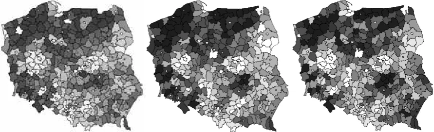
Figure 2: Unemployment in Polishpoviats (Dec 1998 in left panel, Dec 2003 in the middle and Jun 2008
in the right panel, the darker the shade, the higher relative unemployment rate). Source: registry data,
ML&SA
indicating that generallypoviatswith higher unemployment rate are larger (national average is population
weighted), which is depicted by Figure (1). This is an important observation, since generally municipal units are larger than rural ones, but at the same time they typically experience better labour market outlooks (large cities). Consequently, these are larger non-urban local labour markets, which drive this result, suggesting that their employment prospects may indeed be dramatic.
More importantly, as can be inferred from Figure (1), dispersion of the unemployment rates has been constantly growing over the entire time span - especially in the down cycles, be it seasonal effects or general trends in the labour market evolution (the solid line demonstrates the non-weighted average standard deviation for the whole period). This observation suggests that whenever job prospects worsen in general throughout the country, more deprived regions are hit harder. On the other hand, although rather worrying as a labour market phenomenon, this is rather fortunate from the empirical point of view, since overall dispersion both increased and decreased in the analysed time horizon. Therefore, obtained results do not risk to be driven by short term uni-direction trends.
The maps on Figure (2) demonstrate December unemployment rates on poviat level for the 1998,
2003 and the most recent available June 2008, with the shades darkening with the relative labour market hardships. Data demonstrates that the discrepancies on the regional level are even 25-fold (from 0.11 of
the 50% percentile to 2.8 of this value in December 1998)13.
5
Results - distribution dynamics
The analysis ofσ-convergence - as covered in Section 3 - allows to inquire the dynamics of local
unemploy-ment rates distribution. In principle, this analysis may be treated as observing the ”ranking” of poviats
at each point in time and verifying, whether a position in this ranking (measured by the relative distance
to the average) changes or not with respect to previous period ranking. In other words, if allpoviats were
moving towards the average, one would expect a horizontal alignment of the resulting contour plot of the conditional density function (in the ”ranking” the relative distance between the lowest and the highest is
shrinking). Ifpoviats are moving away from the average, one would observe a vertical shape (the relative
distance is growing).
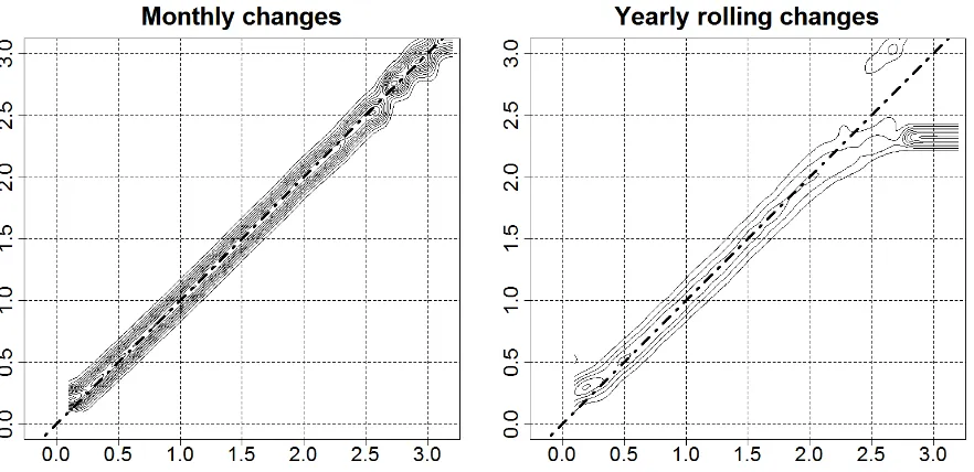
Figure (3) presents contour plots of the density functions showing distribution dynamics for relative
unemployment rates inpoviats over the whole period for which data is available (December 1998 - June
2008) - monthly changes on the left panel and yearly rolling in the right panel14. These figures depict in
two dimensions the distribution of the current relative unemployment rate (vertical axis) conditioned on
13
White spots follow from the changes in the structure ofpoviats in Poland. As of January 2001 municipal units were created, while past data referring to these units cannot be inferred from CSO datasets.
14
the relative unemployment rate in previous period (horizontal axis). Monthly relative unemployment rates seem to be very stable (figure is positioned along the diagonal, which suggests that only small changes in unemployment occur on a monthly basis).
Yearly relative unemployment rate (right panel) shows that more changes occur on yearly basis than on monthly basis, but unemployment is still quite stable (figure is mainly positioned along the diagonal). However there are two peaks on the opposite ends of the figure that seem to position more along the hor-izontal axes - especially the one for the high unemployment rate values. This suggests that separately the
poviats with highest unemployment rates (above 2.3 of the average) and those with lowest unemployment rates (below 0.25 of the average) are becoming similar, so there is an indication of convergence of highest
and lowest unemploymentpoviats separately. Therefore - if any - convergence of clubs may be observed
[image:10.595.84.525.238.452.2]for highest unemploymentpoviats.
Figure 3: Kernel density estimates - levels, NUTS4 units in relation to the national average, 1998-2008.
Source: own calculation based on registry data.
Although ordering ofpoviats seems fairly stable over time, within the last decade only convergence of
clubs could be observed, with high unemployment and low unemployment poles of gravitation. Computing the transition matrices intuitively confirms these findings. Transition matrices report probabilities of moving from one decimal groups to the other calculated at every point in time. They are a discrete equivalent of the kernel density estimates discussed above. At the beginning of the sample (December 1998) poviats were allocated to ten equal sized groups with respect to initial values of the relative unemployment rate. Transition matrix for poviats from each decile group reports probabilitiy of staying in the same decile group or moving up or down the relative unemployment rate scale. This procedure similarly to kernel density estimates was applied for monthly and 12-month rolling changes (left and right panel of Table 1
respectively). 15.
On average 91% ofpoviats remain in the same group on the monthly basis, while 62% are likely not
to change the decimal group for rolled 12-monthly changes. Probabilities above the diagonal are in most cases slightly higher than the ones below, suggesting that moving to higher decimal group (group of higher
15
Table 1: Dispersions - distribution dynamics for relative unemployment rate (transition matrix)
1 2 3 4 5 6 7 8 9 10 1 2 3 4 5 6 7 8 9 10 1 97 3 0 0 0 0 0 0 0 0 88 11 1 0 0 0 0 0 0 0 2 3 92 5 0 0 0 0 0 0 0 15 64 18 3 0 0 0 0 0 0 3 0 5 89 6 0 0 0 0 0 0 1 20 56 20 3 0 0 0 0 0 4 0 0 6 87 6 0 0 0 0 0 0 2 21 48 24 4 0 0 0 0 5 0 0 0 6 87 7 0 0 0 0 0 0 1 23 46 24 5 0 0 0 6 0 0 0 0 7 87 6 0 0 0 0 0 0 3 24 46 23 4 0 0 7 0 0 0 0 0 6 89 5 0 0 0 0 0 0 2 24 52 19 2 0 8 0 0 0 0 0 0 5 90 5 0 0 0 0 0 0 1 18 60 20 1 9 0 0 0 0 0 0 0 5 91 4 0 0 0 0 0 0 0 17 67 16 10 0 0 0 0 0 0 0 0 3 97 0 0 0 0 0 0 0 0 11 89 E 8 8 8 9 9 9 10 11 12 14 9 7 6 7 7 8 9 11 15 22
Notes: Table reports the probabilities in percents. Boundaries for the decimal groups were given by 66.5%, 81.1%, 91.7%, 102.6%, 113.3%, 125.5%, 139.7%, 156.8%, and 180% of the national unemployment rate in the case of monthly transitions. For rolled 12-month transitions these boundaries were 67.3%, 81.3%, 91.7%, 102.3%, 112.9%, 124.7%, 138.4%, 155.6% and 177.9%. In either case, they were computed based on the empirical distributions in the initial period.
LineEdenotes values for ergodic vector.
unemployment) is more likely. Importantly, the majority of transitions on an annual basis happens around
4th to 6thdecimal groups, mostly among themselves. For high unemployment regions the probability of
remaining in the same decimal group reaches 80%-90% thresholds over the analysed period. Generally, out-of-diagonal values are rather small, which suggests that the distribution is very stable. Graphically, this was exhibited by the thickness of the kernel density estimates - they are very thin.
The ergodic values confirm the above statements. Namely, although the size of this effect is not very large, lower unemployment groups loose districts, while the higher ones gain. It is interesting to observe that in case of 12-month transitions (left matrix) the ergodic distribution indicates polarization with relatively stable group of lowest unemployment rate, increasing number of poviats at high unemployment groups and diminishing middle unemployment groups.
Table (2) demonstrates the values of ergodic vectors when one takes into account the structure of
unemployment in Polishpoviats as well as financing and coverage of ALMPs. According to the procedure
Table 2: Dispersions - conditional ergodic vectors
Group 1 Group 2 Group 3 Group 4 Group 5 Group 6 Group 7 Group 8 Group 9 Group 10
Unconditional
Monthly(a) (666.5%) (66.5-81.1%] (81.1-91.7%] (91.7-102.6%] (102.6-113.3%] (113.3-125.5%] (125.5-139.7%] (139.7-156.8%] (156.8-180%) (>180%)
Monthly rolled(a) 9% 7% 6% 7% 7% 8% 9% 11% 15% 22%
Monthly(b)
8% 8% 8% 10% 11% 11% 10% 11% 12% 11%
Conditional
(664.5%) (64.5-77%] (77-86.4%] (86.4-95.8%] (95.8-105.8%] (105.8-116.8%] (116.8-129.2%] (129.2-145.3%] (145.3-165.8%) (>165.8%)
Inflows rate(b) 8% 8% 8% 8% 9% 10% 10% 11% 13% 14%
(664.5%) (64.5-77.1%] (77.1-86.5%] (86.5-96.1%] (96.1-106%] (106-117.1%] (117.1-129.3%] (129.3-145.4%] (145.4-166%) (>166%) Outflows rate(b)
8% 7% 8% 8% 9% 10% 10% 11% 13% 14%
(664.5%) (64.5-77%] (77-86.4%] (86.4-95.9%] (95.9-105.9%] (105.9-116.9%] (116.9-129.2%] (129.2-145.3%] (145.3-166%) (>166%) % of females(b)
8% 8% 8% 8% 9% 10% 10% 11% 13% 14%
(664.5%) (64.5-77%] (77-86.5%] (86.5-95.9%] (95.9-105.9%] (105.9-117%] (117-129.3%] (129.3-145.4%] (145.4-165.9%) (>165.9%)
% of LTU(b) 8% 7% 7% 8% 9% 10% 10% 11% 13% 15%
(664%) (64-76.3%] (76.3-85.1%] (85.1-94%] (94-104%] (104-114.5%] (114.5-127.2%] (127.2-142.4%] (142.4-161.9%) Group 10 (>161.9%)
% of rural inhabitants(b) 18% 14% 12% 12% 10% 9% 8% 7% 6% 5%
(665.9%) (65.9-76.8%] (76.8-86.6%] (86.6-96.4%] (96.4-105.4%] (105.4-115.8%] (115.8-127.5%] (127.5-143.6%] (143.6-162.7%) (>162.7%)
% of female LTU(b) 8% 7% 8% 8% 9% 10% 11% 11% 13% 15%
(664.5%) (64.5-77.1%] (77.1-86.5%] (86.5-96%] (96-106%] (106-117%] (117-129.3%] (129.3-145.3%] (145.3-165.9%) (>165.9%) % of youth(b)
8% 7% 7% 8% 9% 10% 10% 11% 13% 15%
(664.5%) (64.5-76.8%] (76.8-86.4%] (86.4-95.9%] (95.9-105.9%] (105.9-117.1%] (117.1-129.3%] (129.3-145.3%] (145.3-166.1%) (>166.1%)
% of benefits recipients(b) 8% 8% 8% 8% 9% 10% 10% 11% 13% 15%
(665.9%) (65.9-76.8%] (76.8-86.6%] (86.6-96.4%] (96.4-105.4%] (105.4-115.7%] (115.7-127.5%] (127.5-143.6%] (143.6-162.7%) (>162.7%) PLN per treated(c)
4% 4% 4% 6% 8% 9% 11% 13% 18% 23%
(665.9%) (65.9-76.8%] (76.8-86.6%] (86.6-96.4%] (96.4-105.4%] (105.4-115.7%] (115.7-127.6%] (127.6-143.6%] (143.6-162.8%) (>162.8%)
PLN per unemployed(c) 4% 4% 4% 6% 8% 9% 11% 13% 17% 23%
(665.9%) (65.9-76.9%] (76.9-86.7%] (86.7-96.4%] (96.4-105.4%] (105.4-115.8%] (115.8-127.6%] (127.6-143.6%] (143.6-162.7%) (>162.7%)
% of treated(c) 5% 4% 5% 6% 8% 9% 11% 13% 17% 23%
Source: Registry data from CSO and ML&SA. Monthly rolled denotes 12-month changes (annual) rolled over the entire span, where step size is one month. (a)
denotes time period 1998-2008,(b) denotes time sample 2000-2006,(c)denotes time sample 2001-2006
Comparing the results for varied control factors one should note four important points. First of all,
the longer the time span, the more clear emergence of high-end club ofpoviats. This is surprising since, as
depicted by Figure (1), 2007-2008 period saw a stark improvement in the general labour market conditions. Dispersion measured by standard deviation decreased as well. Therefore, clear emergence of these ”clubs” as well as decreasing size of middle-range decimal groups suggest that improvement was not equally spread, while for regions within 20% of the average (both below and above) relative deprivation seems to be suggested by data.
This assertion is further corroborated when one compares the boundaries for conditional and uncon-ditional analyses. Namely, as of third decimal group boundaries are lower in the case of conuncon-ditional. This implies that heteroscedasticity of residuals in each separate regression is inversely linked to the unemploy-ment level. This implies less regions are essentially less ”responsive” to changes in structure, but also policy instruments employed. While justifiable by the nature of unemployment dynamics (local labour markets experiencing more hardship are generally less dynamic and therefore have lower ”disturbancies”),
this finding will impose the necessity to perform β convergence analyses taking into account estimators
consistent in this environment.
Third finding is that in general there is little difference between the ergodic vectors in unconditional and conditional analyses. This suggests that there is no clear answer to the question about the drivers of un-employment rate dynamics. None of the structural factors analyzed seems to have significant explanatory power in as far as differing dynamics are concerned.
The fourth conclusion concerns the fact that essentially none of the financial measures seems to con-tribute to higher cohesion. The size of two high-end groups virtually doubles, while the lowest unem-ployment regions become half as numerous whichever of the measures is concerned. Data do not seem to suggest that financial measures reach their objectives. Naturally, we lack the clear case-specific
counter-factual (what would have happened in each of the units if the financing were not there), but from theex
post perspective they seem to suggest that polarization tendencies are strengthened rather than cohesion.
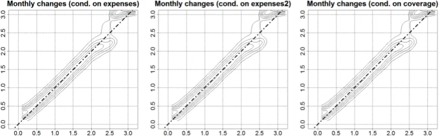
[image:13.595.79.518.469.607.2]This last conclusion is further corroborated by contour graphs depicting the behaviour of conditional kernel density estimates for policy measures, Figure (4).
Figure 4: Kernel density estimates - impact of policy measures, NUTS4 1998-2008. Source: own calculation
based on registry data.
Essentially, unlike in Figure (3), the ”club” of high relative unemployment groups lies above the
diagonal. This is equivalent to stating that they converge tohigher unemployment levels when controlling
for the effect of policy instruments. In other words, had the financing been not accounted for, the behaviour
of the data suggested convergence towardslowerlevels. Although this may suggest that policy instruments
are in fact counterproductive, this finding may also result from the nature of the financing algorithm. As was described earlier, local labour markets suffering more absolute and relative hardships receive more financing. We are unable to analytically discriminate between these two explanations, while probably both effects are at play.
within the high and low unemployment poles of gravitation do not necessarily have to be neighbouring
or close geographicallypoviats, while the specific processes might differ significantly in the underpinnings.
As maps demonstrated in Figure (2) suggest, that in fact this is the case, i.e. there are regions where poor
labour market performance spreads across thepoviats(North and especially northern West). At the same
time improvements in relative local unemployment rates seem to have two main roots. On one hand, they follow from a statistical artefact: the increase of the overall average with the constant local unemployment rate leads to lower relative rate - in fact, labour market situation in real terms did not improve in these
particular poviats. Alternatively, improvements may owe to the idiosyncratic positive shocks due to, for
example, localisation of new investments (cfr. Gorzelak (1996)).
All analyses in this sections consider distribution dynamics, i.e. evolution of relative unemployment
rates. Their levels - if used at all - served the purpose of ”grouping” poviats. However, the severity
of the unemployment problems follows not only from the distribution, but from the magnitude of this phenomenon too. To address this problem we analyse the convergence in levels of unemployment.
6
Results -
β
convergence
In this section we report the results of a panel regression of unemployment growth in periods t on the
unemployment in the initial period (the β-convergence). To control for low and high unemployment
regions, a synthetic proxy was generated, indicating to which of the ten decimal groups a poviat belong
in the initial period. Since this measure is constructed on the basis of empirical distribution moments, it can take simply the values of 1 to 10, without hazarding the correctness of estimates due to non-linear or non-monotonic effects. In the estimation a dummy correcting for the statistical effect of December 2003 was additionally included. To control for seasonality as well as changing labour market conditions, overall unemployment rate in Poland was incorporated, although from an econometric point of view introducing this variable plays the role of imposing fixed effect on period in the cross-sectional time-series analysis. Finally, some interaction terms were allowed for, to see the extent to which initial distribution and initial unemployment rate effects are symmetric for high and low unemployment regions. Consequently, the following equation was under scrutiny:
unemploymenti,t =α+β·unemploymenti,T0+γ·control variablesi,t+ǫi,t. (5)
This equation was estimated in a number of versions. Naturally, we first approach the unconditional
form ofβconvergence, but this may be approached in at least two ways. One of them comprises comparing
initial states with composite changes throughout the entire time span (∆unemploymenti =ui,T −ui,t,
where t = Dec1998 and T = J un2008). Another way is to make use of rolling estimates using, for
example, 12-month changes. Consequently, one would consider ∆unemploymenti=ui,t−ui,t−12. Moving
to conditional form of convergence, one can include control factors (structure and dynamics of local labour
markets16) as well as policy variables (intensity, depth and extensiveness of ALMPs). Naturally, this can
only be done in a rolling version. Including structural and policy variables limits sample for the reasons of data availability. Including 12-month lags and differences deprives the analysis of an additional year, leaving 60 periods per unit.
To asses that local unemployment rates exhibitβ-convergence, the coefficient ofβin equation (5) would
need to turn out statistically significant and below unity. Value of this coefficient exceeding unity would suggest divergence in levels. However, one must keep in mind that the period we analyse was characterised by stark increase of the unemployment rates, while the final level (June 2008 ) was only approaching the initial one (December 1998) for most of the observations. Therefore, exceeding unity size of estimator
in the unconditional version would only be a confirmation, thatpoviats with higher unemployment rate
in the initial period observe higher unemployment growth rates in subsequent periods - not necessarily
that the response is asymmetric among poviats. This is why additionally we include national average
16
unemployment rates in the estimations. Please note, that it is equivalent to having time-specific fixed effects in the analysis.
Monthly data (relatively high frequency) may exhibit seasonality and autocorrelation. In addition, since units of analysis differ substantially in unemployment levels and changes observed over time, one risks heterogeneity as well. Therefore, our preferred econometric specification is feasible generalised least squares (FGLS) with heteroscedasticity and autocorrelation consistent standard errors and panel-specific autocorrelation structure. On the other hand, however, there are strong arguments in favour of the potential endogeneity. Namely, although financing of the ALMPs follows a backward looking algorithm, if underlying fundamentals exhibit persistence - which they frequently do - statistical issues emerge. The best way to circumvent the potential bias of the estimators is to use the GMM as developed by Arellano and Bond (1991). However, standard estimators do not permit autocorrelation. Therefore, we resort to an estimator consistent under autocorrelation, as developed by Arellano and Bover (1995) and Blundell and Bond (1998).
Table 3: Levels -β convergence analysis
(1) (2) (3) (4) (5) (6) (7) (8) (9) (10) (11)
Initial unemployment 1.037*** 0.24*** 0.13*** 0.28***
ui,t0 (0.033) (0.007) (0.02) (0.009)
Initial unemployment 0.81*** 0.89*** 0.89*** 0.89*** 0.88*** 0.88*** 0.87*** 0.75*** 0.46*** -0.66***
ui,t−12 (0.001) (0.002) (0.002) (0.002) (0.003) (0.003) (0.004) (0.005) (0.011) (0.006)
% of females -6.99*** -4.39*** -5.58*** -4.24*** -11.34*** -7.55***
(0.36) (0.38) (0.45) (0.44) (0.61) (0.61)
% of LTU -0.92*** -1.18*** -2.25*** -1.45*** -1.24*** -0.86***
(0.12) (0.11) (0.14) (0.14) (0.22) (0.18)
% of youth 2.93*** 3.26*** 3.26*** 2.91*** 3.57*** 0.96**
(0.27) (0.27) (0.30) (0.30) (0.42) (0.4)
% of rural -1.47 -1.33 -1.42 -1.48 -1.32 -1.27
(1.29) (1.22) (1.09) (1.12) (1.15) (1.97)
% of 50+ -2.75*** -3.08*** -3.33*** -3.12*** -2.88*** -2.98***
(0.20) (0.20) (0.23) (0.23) (0.32) (0.29)
Inflows rate -8.07*** -7.31*** -9.12*** -9.61*** -6.54*** -10.96***
(0.49) (0.48) (0.56) (0.57) (0.69) (0.72)
Outflows rate -15.19*** -14.16*** -14.28*** -17.61*** -14.99*** -20.13***
(0.72) (0.68) (0.79) (0.81) (1.02) (1.00)
% of treated -0.10* -0.11* -0.10* -0.16** -0.22***
(0.071) (0.074) (0.074) (0.09) (0.09)
Exp. per unemployed -0.09 -0.09 -0.09 -0.09 -0.136
(0.07) (0.06) (0.065) (0.07) (0.08)
Exp. per treated -0.09 -0.09 -0.085 0.017 -0.16**
(0.06) (0.06) (0.06) (0.07) (0.07)
Time trend No No Yes Yes Yes Yes Yes Yes Yes Yes Yes
No of observations 374 36 694 36 694 29 185 29 186 29 185 22 719 22 719 21 211 5 983 15 228 Estimation technique
χ2 594.8*** 2450.6*** 67109.3*** 39216.03*** 30127.5*** 40685.29*** 20642.8*** 31135.2*** 30621.3*** 11614.2*** 25961.2*** Notes: GMM estimators with robust standard errors. Robust standard errors reported. Time trend, linear and squared, significant (not reported, available upon request).
Standard errors in parentheses. *, ** and *** denote statistical significance at 1% 5% and 10% levels, respectively. Except for pooled unconditional estimation (first column),χ2Wald statistics highly statistically significant,p-valuesavailable upon request.
Column (1) of Table (3) reports the analysis for clear formβ-convergence analysis. Namely, we regress the change in unemployment rates over the entire time-span on the initial (December 1998) rate of un-employment. Clearly, no evidence of convergence is provided by the data, the estimator is statistically insignificant. However, taking into account the evolution in national unemployment average one could sus-pect that these 9.5-years changes in unemployment level may be indeed a misleading indicator. Therefore,
in column (2) we move to using rolling version ofβ-convergence analysis. Namely, we use 12-month lags as
”initial” unemployment level and 12-month differences as changes in unemployment, while the estimates are calculated over the entire sample. Findings are slightly more optimistic in a sense that statistically sig-nificant negative coefficient is found. The size of this estimator decreases slightly when we introduce time trend (both linear and squared), as reported in column (3). The inclusion of trend improves the statistical properties of the model, whilst it is also justified by the evolution of the national average unemployment rate, as depicted by Figure (1).
Columns (4)-(8) report conditional β-convergence analyses for the entire available sample. We first
control for the local unemployment structure (female share of unemployed, the share of long-term unem-ployed, youth as well as workers above 55 years of age and workers inhabiting rural areas). We include here also measures of local labour market dynamics (inflows and outflows rates). Although these may be affected by policy instruments (e.g. providing financial incentives to registration by relaxing the require-ments or offering more activisation opportunities), they are to a much higher extent a factor discriminating between ”sleepy” and ”active” labour markets. All these variables turn out significant and with expected signs. Estimators of structural variables are also fairly stable across the specifications, which suggests they
are not correlated well with variables at the core of interest in this paper,i.e. policy instruments.
Columns (7) and (8) report estimators for measures of availability of financing, average treatment
cost as well as treatment coverage (per se and controlling for unemployment structure and dynamics,
respectively). In column (7) neither intensity nor extensiveness of active labour market policies prove significant in the estimations. When unemployment structure is controlled for, the estimator of financing availability changes its sign, while coverage remains insignificant. Average treatment cost receives the same, negative sign as availability of financing. These estimators remain stable across further specifications.
The conclusions thusfar imply, that policy instruments have the same direction of the effect as more unfavourable characteristics of unemployment structure. In general, the only structure variable entering with a positive sign was the share of youth among unemployed, while this is exactly the group with comparably lowest hardships when compared to elderly, inhabiting rural areas or long term unemployed. As to the estimator of female share, its negative sign is consistent with the analyses made on Labour Force Survey data, demonstrating that gender discrimination is observed to a lesser extent in wages and to a higher extent in labour market access.
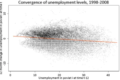
Column (9) reports the same regression results as column (8) with the main difference being the inclusion of initial (December 1998) unemployment rate. Technically, this plays the role of a panel specific fixed effect estimator for a constant. The estimator is significant and has a positive sign, which suggests
that in fact convergence is weaker among poviats with initially more hardships. The negative coefficient
ofui,t−12coefficient is only marginally larger than that ofui,t0, which implies thatde factoconvergence is
much weaker than suggested by the relatively large size of estimator from the previous estimations. This is depicted on Figure (5).
Finally,σ-convergence analysis suggested that in as far as the behaviour of univariate regression
resid-uals are concerned, lowest three decimal groups display different characteristics than the majority of the sample. Therefore, we performed the analysis as in column (9) for two separate sub-samples: three lowest decimal groups in column (10) and the reminder in column (11). This step was taken to observe if these groups would differ in the sign of influence of policy instruments on regions experiencing less hardship
Figure 5: Convergence of unemployment levels, 1998-2008. Source: own calculation based on registry data.
of instruments used in more favoured regions. This is striking because one would typically associate lower unemployment with large, fast growing cities and higher level of human capital, including the level of local public employment services performance. Results seem to show consistent negative impact, while there seems to be more diversity (more good performance and bad performance labour offices) in the reminder of the sample.
Conclusions from this part of analysis suggest that even though we could find some statistical support to the hypothesis of convergence in levels, it is (i) weak, (ii) weaker among higher initial unemployment regions and (iii) independent or negatively affected by active labour market policy measures.
7
Conclusions
For most analyses of convergence one experiences a difficulty of no clear counterfactual, (Boldrin and Canova 2001). The literature traditionally assumes that diversification of the use and coverage of cohesion policies provides sufficient variation to derive conclusions regarding the effectiveness of cohesion efforts. The main purpose of this paper was to inquire the convergence patterns of local labour markets in a transition economy, analysing the effects of policy instruments. We used policy relevant NUTS4 level data, since actual labour market policies - with special emphasis on the active ones - are performed at exactly this level. Time span in this study allows to cover both up and down cycles in labour market conditions, which guarantees that the results are not trend driven.
In order to inquire the nature of the local unemployment rates evolution we employed parametric
econometric techniques (convergence of levels, β-convergence) as well as nonparametric kernel density
estimates (convergence of dispersion,σ-convergence). The distribution of unemployment rates in Poland
was found to be highly stable over the sample period with only minor evidence in support of the convergence
of clubs - high unemployment poviats. In addition, data support only weak conditional β-convergence,
policies contribute to cohesion. In fact, we find that if one statistically controlls for the effects of policies, divergence is more apparent. Policy measures are proxied in our study by the extensiveness and intensity of active labour market policies financing (expenses per one unemployed and expenses per one person in treatment) as well as their depth (coverage of treatment).
Unfortunately, sample commences already some years after the transition, which makes it impossible to establish a direct link between transition and local unemployment rate dynamics. On the other hand, our findings suggest that whenever job prospects get better all the way through the country, already disadvantaged regions benefit less in each of the examined countries. Therefore, the time-span is relatively
short, especially in the context of stochastic convergence studies in the literature17. Consequently, our
results should be interpreted with caution.
On the other hand, our findings are consistent with earlier study by Gora, Lehmann, Socha and Sztanderska (1996). However, our interpretation of these findings differs in a sense that we do not attempt to judge the adequateness of separate instruments used, rather the overall quality of PES performance. Naturally, weak evidence of convergence may be interpreted in wider terms of general conclusion that such measures do not work. We share the view that in order to provide such strong conclusions one should be first confident that value for money ratio is fairly rational. Currently, local labour offices receive financing irrespectively of their performance. Consequently, distribution of financing does not constitute an incentive for offices to improve performance while spending the available budget is is the main area of evaluation by NUTS2 authorities as well as Ministry of Labour and Social Affairs. Each of the Polish NUTS2 regions contains districts from highest unemployment groups. Should financing be geared towards alleviating the situation in most deprived regions by fostering higher effectiveness, altering the impact on convergence might be expected.
References
Arellano, M. and Bond, S.: 1991, Some Tests of Specification for Panel Data: Monte Carlo Evidence and
an Application to Employment Equations,Review of Economic Studies58(2), 277–97.
Arellano, M. and Bover, O.: 1995, Another Look at the Instrumental Variable Estimation of
Error-components Models,Journal of Econometrics68(1), 29–51.
Armstrong, H. and Taylor, J.: 2000,Regional Economics and Policy, 3rd edn, Blackwell.
Barro, R. and Sala-i Martin, X.: 2003,Economic Growth, MIT Press.
Bayer, C. and Juessen, F.: 2006, Convergence in West German Regional Unemployment Rates.
Bianchi, M. and Zoega, G.: 1999, A nonparametric Analysis of Regional Unemployment Dynamics in
Britain,Journal of Business & Economic Statistics17(2), 205–216.
Blanchard, O. and Katz, L.: 1992, Regional Evolutions,Brookings Papers on Economic Activity1(1), 1–75.
Blundell, R. and Bond, S.: 1998, Initial Conditions and Moment Restrictions in Dynamic Panel Data
Models,Journal of Econometrics 87(1), 115–143.
Boeri, T. and Terrell, K.: 2002, Institutional Determinants of Labor Reallocation in Transition, Journal
of Economic Perspectives16(1), 51–76.
Boldrin, M. and Canova, F.: 2001, Inequality and Convergence in Europe’s Regions: Reconsidering
Euro-pean Regional Policies,Economic Policy 16(32), 205–253.
17
Buettner, T.: 2007, Unemployment Disparities and Regional Wage Flexibility: Comparing EU Members
and EU-accession Countries,Empirica34, 287–297.
Camarero, M., Carrion-i Silvestre, J. L. and Tamarit, C.: 2006, Testing for Hysteresis in Unemployment
in OECD Countries: New Evidence Using Stationarity Panel Tests with Breaks,Oxford Bulletin of
Economics and Statistics68(2), 167–182.
Carlino, G. A. and Mills, L. O.: 1993, Are U.S. Regional Incomes Converging? A Time Series Analysis,
Journal of Monetary Economics32(2), 335–346.
de la Fuente, A.: 2000, Convergence Across Countries and Regions: Theory and Empirics,CEPR
Discus-sion Papers 2465, Centre for Economic and Policy Research.
Decressin, J. and Fatas, A.: 1995, Regional labor market dynamics in Europe,European Economic Review
39(9), 1627–1655.
Egger, P. and Pfaffermayr, M.: 2005, SpatialβandσConvergence: Theoretical Foundations, Econometric
Estimation and Application to the Growth of European Regions. Spatial Econometrics Workshop, Kiel, Germany.
Ferragina, A. M. and Pastore, F.: 2008, Mind the Gap: Unemployment in the New EU Regions,Journal
of Economic Surveys22(1), 73–113.
Fihel, A.: 2004,Polscy pracownicy na rynku Unii Europejskiej (Polish Workers in EU Labour Markets),
Wydawnictwo Naukowe Scholar, chapter Aktywno´s´c ekonomiczna migrant´ow na polskim rynku pracy, pp. 115–128.
Gomes, F. A. R. and da Silva, C. G.: 2006, Hysteresis vs. Nairu and Convergence vs. Divergence: The
Behavior of Regional Unemployment Rates In Brazil,Technical report.
Gora, M., Lehmann, H., Socha, M. and Sztanderska, U.: 1996,Labour Market Policies in the Transition
Countries: Lessons from their Experience, OECD, Paris, chapter Labour Market Policies in Poland: An Assessment.
Gorzelak, G.: 1996, The Regional Dimension of Transformation in Central Europe, Jessica Kingsley
Publishers London.
G´ora, M. and Lehman, H.: 1995, How Divergent is Regional Labour Market Adjustment in Poland?,
in S. Scarpetta and A. W¨org¨otter (eds), The Regional Dimension of Unemployment in Transition
Countries. A Challenge for Labour Market and Social Policies, OECD.
Grotkowska, G.: 2006, The Case of Poland - Recent Changes of Non-standard Employment and Labour
Market Flexibility,inC. Kohler, K. Junge, T. Schroder and O. Struck (eds),Trends in Employment
Stability and Labour Market Segmentation, SFB 580 Mitteilungen, Universitat Jena.
Huber, P.: 2007, Regional Labour Market Developments in Transition: A Survey of the Empirical
Litera-ture,European Journal of Comparative Economics4(2), 263 – 298.
Kaczmarczyk, P. and Tyrowicz, J.: 2008, Wsp´olczesne procesy migracyjne w Polsce (Contemporaneous
Migration Processes from Poland), Fundacja Inicjatyw Spoleczno-Ekonomicznych, Warszawa.
Lehmann, H. and Walsh, P.: 1998, Gradual Restructuring and Structural Unemployment in Poland: A Legacy of Central Planning. mimeo, LICOS, Centre for Transition Economies, Katholieke Universiteit Leuven, Leuven.
Lopez-Bazo, E., del Barrio, T. and Artis, M.: 2002, The Regional Distribution of Spanish Unemployment:
Lopez-Bazo, E., del Barrio, T. and Artis, M.: 2005, Geographical Distribution of Unemployment in Spain,
Regional Studies39(3), 305–318.
Marelli, E.: 2004, Evolution of employment structures and regional specialisation in the EU, Economic
Systems28(1), 35–59.
M¨unich, D., Svejnar, J. and Terrell, K.: 1997, The Worker-Firm Matching in the Transition: (Why) Are
the Czechs More Successful than Others?,Working Paper 107, The William Davidson Institute.
Munich, D., Svejnar, J. and Terrel, K.: 1998, Worker-Firm Matching and Unemployment in Transition
to a Market Economy: Why Are The Czechs More Successful Than Others,University of Michigan
mimeo.
Newell, A. and Pastore, F.: 1999, Structural Unemployment and Structural Change in Poland, Studi
Economici69(3), 81–100.
Obstfeld, M. and Peri, G.: 1998, Regional nonadjustment and fiscal policy: lessons from EMU, NBER
Working Paper 6431, NBER.
Overman, H. and Puga, D.: 2002, Regional Unemployment Clusters,Economic Policy17(34), 117–147.
Paas, T. and Schlitte, F.: 2007, Regional Income Inequality and Convergence Processes in the EU-25. Nordic Econometric Meeting, Tartu, Estonia.
Perugini, C., Polinori, P. and Signorelli, M.: 2005, GDP Growth and Employment in EU’s Member
Regions: Convergence Dynamics and Differences for Poland and Italy,EACES Discussion Paper 2,
EACES.
Pritchett, L.: 1997, Divergence, Big Time,Journal of Economic Perspectives11(1), 3–17.
Quah, D. T.: 1996, Twin Peaks: Growth and Convergence in Models Distribution Dynamics, Economic
Journal106(437), 1045–1055.
Scarpetta, S. and Huber, P.: 1995, Regional Economic Structures and Unemployment in Central and
East-ern Europe. an Attempt to Identify Common PattEast-erns,The Regional Dimension of Unemployment
in Transition Countries. A Challenge for Labour Market and Social Policies, OECD.
Silverman, B.: 1986,Density Estimation for Statistics and Data Analysis, Chapman &Hall.
Sims, C. A.: 1972, Money, Income and Causality,American Economic Review62(4), 540–552.
Svejnar, J.: 2002a, Labour Market Flexibility in Central and East Europe, William davidson institute
working paper, William Davidson Institute.
Svejnar, J.: 2002b, Transition Economies: Performance and Challenges,Journal of Economic Perspectives
16(1), 3–28.
Sztanderska, U. and Socha, M.: 2001,Strukturalne podstawy bezrobocia w Polsce (Structural Character of
Unemployment in Poland), PWN, Poland.
Temple, J.: 1999, The New Growth Evidence,Journal of Economic Literature37(1), 112–156.
Tyrowicz, J.: 2006, Organizacje pozarzadowe na rynku pracy: unikatowe grupy czy universalne
kompe-tencje? (ngos in the labour market services: Unique groups or universal competences?),inM. Boni,
I. Gosk, B. Piotrowski, J. Tyrowicz and K. Wygnanski (eds), Rola organizacji pozarzadowych na