Multi Sensor Context Aware Clothing

Multi-Sensor Context Aware Clothing

Kristof Van Laerhoven, Albrecht Schmidt and Hans-Werner Gellersen

Ubicomp Group

Lancaster University

LA1 Lancaster 4YR, United Kingdom

{kristof, albrecht, hwg}@comp.lancs.ac.uk

Abstract

Inspired by perception in biological systems, distribution of a massive amount of simple sensing devices is gaining more support in detection applications. A focus on fusion of sensor signals instead of strong analysis algorithms, and a scheme to distribute sensors, results in new issues. Especially in wearable computing, where sensor data continuously changes, and clothing provides an ideal supporting structure for simple sensors, this approach may prove to be favourable. Experiments with a body-distributed sensor system investigate the influence of two factors that affect classification of what has been sensed: an increase in sensors enhances recognition, while adding new classes or contexts depreciates the results. Finally, a wearable computing related scenario is discussed that exploits the presence of many sensors.

1.

Introduction

The justification for using sensors in a wearable computing architecture ranges from use in intelligence augmentation (such as availability of a real-time clock and calendar, the exact room temperature, or CO-level) to automating tasks depending on particular features of the environment, situation or context (light level driving brightness of the display, temperature sensors regulating heat elements in the clothes [9], stick-e-notes [3], context aware tour guides [6], etc.). Regardless of whether these applications would be sought after by a large community, one trend that can be observed is that sensors are gradually becoming part of mobile and wearable devices. The goal of this paper is to characterize the use of a multitude of simple sensors, and the consequences of focusing on sensor-fusion instead of sensor-specific pre-processing algorithms (such as image- or sound analysis). The idea takes encouragement from perception

in biological organisms, where massively parallel neural pathways maintain a robust flow of sensed impulses to the brain [2].

Distribution of sensors fits to a great degree in research that augments mundane objects with computing elements, commonly referred to as ubiquitous computing. Wearable computers are no exception to this concept either, since large surfaces of clothing are an ideal supporting platform for a multitude of sensors, provided they are miniaturized so that they do not obstruct the wearer. This size constraint often means that the quality of the sensor itself is compromised as well, which leads to the concept of many simple sensors [15].

Once the choice has been made to employ many sensors, two fundamental approaches of where to fuse the sensor data appear: (1) distributed across a network or (2) centralized. After a description of both, we give a motivation for our choice of architecture for the paper’s experiment, which attempts to characterize the impact of both contexts and sensors on the quality of context awareness.

2.

Multi-sensor networks

Finding the optimal way to interconnect many sensors in a network is still an unresolved issue in ongoing research. We distinguish approaches to collect and manage sensor data in large networks in two classes, based on how and where the data is fused. The first uses a tree-like hierarchy to assemble high-dimensional vectors at the root, so they can be fed into a classification algorithm that assigns a description to each input. The latter alternative processes the sensor data locally and then communicates further data to propagate throughout the entire network.

2.1. Centralized processing

Most sensor architectures tend to stream all data, sometimes pre-processed, to one central location. The ease of implementation compared to a decentralized approach and the fact that most systems are inherently based on a single computer anyway, are most likely the prime reasons for this choice.

Figure 1. Centralized processing and fusion of the data.

2.2. In practice: the 30-accelerometer board

Many approaches use some kind of bus to distribute data across a network and increase the number of sensors. The problem with this approach is an extra level of complexity: additional bus-communication requires a microcontroller per sensor(-module) or at least extra complexity in the sensor’s chip-design.

Instead, we opted to optimize our current approach depicted in Figure 1 by increasing the number of sensors for one microcontroller to its absolute maximum without additional components (such as multiplexers / demultiplexers). By utilizing all of the Microchip PIC 16F877 microprocessor’s input channels, we come to a maximum of thirty sensors that can be read and forwarded to a central processor or a hub via a traditional serial port. Since most standard computing platforms support at least four serial ports, 120 sensors could be attached without additional (custom-built) hardware. Of all sensor signals, 8 use the analog outputs of the ADXL202E to be converted to digital inside the microprocessor, and the other 22 use the Pulse Width Modulation (PWM) outputs to connect to the microprocessor’s digital input pins. Figure 2 depicts the internals of the sensor board. The remainder of this paper will specify accelerometers as the used sensors, the type we use (ADXL202E dual axis accelerometers from Analog Devices) outputs the acceleration in both analog and PWM.

Figure 2. The PIC-based sensor-reading module, able to read thirty sensor values at once and stream them to the RS232 serial port. Right are a few of the accelerometers.

// read PWM0

if (bad[0]<bad_buffer) { high = 0;

while(input(PIN_C0)&&

(high<bad_overfl) )

{ high++; } // wait until low

if (high>(bad_overfl-1)) { bad[0]++; }; high = 0;

while(!input(PIN_C0)&& (high<bad_overfl) )

{ high++; } // wait until high

if (high>(bad_overfl-1)) { bad[0]++; }; high = 0;

while(input(PIN_C0)&&

(high<bad_overfl) )

{ high++; } // count high-time

if (high>(bad_overfl-1)) { high=0; bad[0]++; } val[8] = high;

}

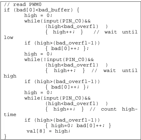
Table 1. Part of the microcontroller’s source code that converts the pulses on pin C0 into an acceleration value.

The design of the printed circuit board (PCB) 1 of this setup contains mainly the microprocessor and an array of

The PCB, schematics, and the PIC microprocessor’s source code are publicly available at this website:

http://www.comp.lancs.ac.uk/~kristof/notes/thirtyacc/

se

n

so

rs

se

n

so

rs

hub or processor

Dataflow controller

connectors each providing power, ground, and two input channels for the acceleration sensors. The source code for the microprocessor is straightforward as well, converting the PWM and analog values to digital and printing it to the serial port. Table 1 contains a fragment of the source code in C to read one PWM value. The system waits until the most recent pulse ends, or until the counter (designated as ‘high’ since it counts how long the pulse remains in the high state) crosses a pre-defined maximum value (‘bad_overfl’).

To increase the frequency of reading, time-out values (‘bad_buffer’) on the microprocessor check whether a sensor is still alive and should be polled in the next interval. This technique makes it possible to output 10-bit values for each sensor at 30 samples per second in the worst case (i.e. no PWM-based sensors are connected). A drawback is a slight slowdown in the output stream whenever the time-out values reset, which only becomes noticeable if most sensors are not connected or do not give a proper signal.

2.3. Distributed processing

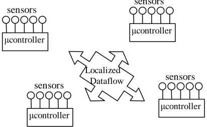
Decentralized sensing is a research field that is getting increasingly more attention (see [10] or [5]). An obvious advantage is the increased robustness of the network compared to the centralized approach: not just sensors, but also entire components can malfunction without failure of the entire system. In some distributed networks, nodes can also be more flexible: they can be introduced, moved, and removed in the network without having to reinitialize all nodes for the new topology. It is beyond the scope of this paper to go into detail about routing techniques in these networks or the specific implementation of communication (wired versus wireless, broadcasting, etc.) for which we refer to [1], [11], or [8].

Figure 3. Distributed processing of the sensor data.

The main focus is on communication or interaction between nodes of the network, instead of fusion of all

data in one place, and an emergent self-organisation between the nodes.

Processing the data in a distributed manner shows also potential in avoiding the fusion of a multitude of sensor data at once, and adding units would be cost-effective since it would mostly involve duplicating the basic design.

2.4. Example: Distributed clustering

In more theoretical work concentrating on the self-organization within a network of sensor modules, a distributed version of the Kohonen Self-Organizing Map was implemented for clustering of the sensor data. The experiment was based on sensor modules from the Smart-Its Project [13], which contain basic sensors (microphone, accelerometers, light sensor, pressure sensor, and thermometer), wireless communication, and basic processing (PIC-based microcontroller). Five Smart-Its modules were spread on a table while their common environment was altered by switching the light on or off, increasing the ambient temperature, and by introducing (audio) noise. Each sensor-module would then specialize itself to one of these states, using the Kohonen learning rule and thus forming a topological cluster network. Results and implementation details can be found in [4].

le arning rate = 0.05

0 50 100 150 200 250

1 105 209 313 417 521 625 729 833 937 1041 1145 1249 1353 1457 1561 1665 0 1 2 3 4 5 6

error winner

Figure 4. Local error (left Y-axis) and winning unit IDs (right axis) over time of the Self-Organizing Map. Units specialize themselves for different states of the environment: lights on (1-330), talking people nearby while lights remain on (331-400), lights turned off (401-800), talking people nearby while light remain turned off (801-1000), and heating on (1090-1400). Source: [4].

2.5. Rationale

Scaling up the number of sensors for a wearable system is not straightforward, as can be deduced from the fact that few systems go over the 10-sensors barrier. Although sensing and communication on distributed platforms is currently available, we chose in our experiments to keep on using the traditional approach controller

controller sensors

sensors

Localized Dataflow

controller sensors

where one microprocessor digitizes the outputs of the sensors and then sends them for further processing to a serial output.

The primary motive for this choice is simplicity. Despite the feasible form factor of the distributed units for wearability, problems related to separate batteries and wireless communication make it a bad choice for forwarding the sensor values to a processor. However, if the required (pre-) processing could be done on the units themselves, distributed processing should be the preferred means for several reasons:

• Scalability has in this paper proven to be an important factor for the quality of recognition. The distributed processing architecture would not need as much reconfiguration affecting the whole network. • Flexibility is an important issue if the assumption is

made that the sensors should be embedded in clothing (which this paper does). People tend to remove, change, and add clothing regularly during the day (and night), which leads to reconfiguration in the sensor network.

• Robustness is for the same reason a requirement since clothing will be washed and could be handled roughly, which could result in breaking sensor modules.

3.

Characterization of Multi-Sensor

Classification

One of the assumptions made in [15] was that increasing the number of sensors would enhance the recognition and classification of contexts. As we now have a truly multi-sensor hardware platform at our disposal, several experiments will test this claim. We will first start with further implementation details based on the hardware that was introduced in the previous section. After showing what the sensor data looks like and how it can be visualized, this wearable setup is put to use in an empirical study on the parameters that influence context awareness.

3.1. A Multi-Accelerometer Outfit

Using the hardware described in section 2.1.1., we are able to integrate thirty accelerometers into a wearable arrangement (depicted in Figure 6). The available accelerometers were spread over the body with the majority on the legs (16) and the rest divided over the arms and upper body (14). The accelerometers for the legs were integrated into a harness to enable testing and capturing of data from multiple users of different figure heights, while the others are attached on regular clothing using Velcro.

Figure 5. The 30-accelerometer module with the harness and all sensors attached: eight accelerometers are distributed over each leg, close to the joints; the other 14 sensors are situated on the upper body and arms.

3.2. A First Look at the Data

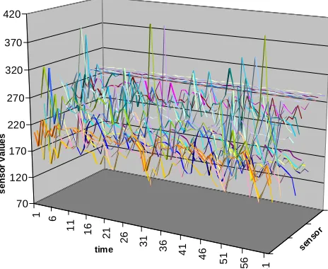
Traditional visualization techniques for the sensor data become inadequate as the number of sensors increases, even when plotting to a three-dimensional series space. Figure 6 for example, shows a time-series plot of the 30 body-worn acceleration sensors while the wearer is walking. Even if we were to provide more details on what accelerometers are positioned where on the body, this plot would be of little use apart from a very coarse-grained classification in amount, speed and patterns of movement.

1 ₆

1

1

1

6

2

1

2

6

3

1

3

6

4

1

4

6

5

1

5

6

6

1

S6 S11 S16 S21 S26

70 120 170 220 270 320 370 420

s

e

n

s

o

r

v

a

lu

e

s

time sen

sor

3.3. Classification Characteristics

We treat context awareness here as a classification of sensor data by a given algorithm, trained by example. The output of this algorithm is a probability or confidence value that states how certain it is that the system is in a certain context, given the data that originated from the sensors. This section is an attempt to identify the parameters that affect the quality of context awareness, regardless of the algorithm that was chosen to do the mapping from sensor data to context:

Quality of sensors. The output quality and resolution of sensors is clearly an important factor in recognition, as they determine the distance (according to an appropriate metric) between sensor data from two contexts in input space. When the sensor values are more precise, contexts are more likely to be distinguished. Furthermore, it is obvious that the choice between two sensors with the same function will result in the more reliable one.

Number of sensors. A first less-examined influence on the quality of context awareness is the number of sensors. While concentrating on just the number of sensors (and thus not on the classification algorithm or robustness of the system), one could argue that including just the sensors that pick up the characteristic aspects of a context will be sufficient and adding sensors will not improve the recognition. However, sensor fusion theory [7] shows that recognition often becomes faster and more accurate as sensors get added.

This leaves us with a few remaining questions: Is it really worth adding sensors to a system? (i.e. we want a quantification of the added value) And how much does the recognition improve per added sensor? The first question depends on case-specific properties such as the complexity of the system, the contexts to be recognized, and the application. However, we can answer the second question by examining the performance of classification as a function of the number of sensors.

Complexity of contexts. Not all contexts are equally easy or hard to recognize. Contexts are often related to one or more concepts that can be perceived by sensors: “walking” gives certain motion patterns for body-worn sensors, or “in the sun” might be recognized by the presence of a certain level in light and increase in temperature. The context “in a meeting” on the other hand, might be distinguished from other contexts by features in the signals coming from microphones and/or presence of people, but is in general much harder to characterize.

Number of contexts. The number of contexts to be distinguished is an often overlooked factor in context awareness. Statistically, the bigger the set of candidate contexts gets, the more chance there is that the algorithm’s prediction will be wrong. We will test this theory on real-world sensor data by monitoring the recognition as the number of contexts goes up.

3.4. Evaluation

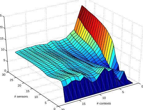
A combination of the two promises made in 3.3 (in italics) should give an indication how any context aware application could behave under a changing number of sensors and recognizable contexts. Using 20 motion-related contexts and the previously mentioned 30-accelerometer system, a 3D plot (Figure 9 and 10) was made with the following axes:

• The X-axis showing the number of sensors used, starting with the best discriminating sensor (based on variance), and adding the next-best sensor until all 30 sensors were used, for each set of contexts (calculated as described in the Y-axis section). • The Y-axis showing the number of contexts to be

distinguished, starting with one context, then adding the best distinguishable next context until all 10 contexts are included.

• The Z-axis contains the degree of dispersion for each set of contexts. The dispersion measure states how dissimilar the data from two contexts really is, and thus indicates how well algorithms could distinguish them. This will obviously be 100% for one context, and decreases as more contexts are added.

150 200

250 300

350 400

150 200 250 300 350 180 200 220 240 260 280 300 320 340

kick right jumping kick left

waving right

kneeling right

kneel left

running kneeling

walking lying on back sit legs bend

standing sit crossed

lying on right sitting chair handstand left up sit stretched

handstand handstand right up

We generalize dispersion here as the distance between the sensor data that is coming from two or more different contexts, not just a degree of spread among data from one class. Figure 8 shows an example where two-dimensional data from two contexts (distinguished by their colour, black or white) has either a high or low dispersion.

Figure 8. Dispersion of sensor data for two contexts, black and white, and how it relates to performance of a context awareness algorithm: (1) a large dispersion indicates that algorithms can easily distinguish the two contexts, while (2) a small dispersion suggests the opposite. The data is visualized by circles, while the means of both data sets are designated by crosses.

Plotting the data in this fashion allows evaluation of the effect that the number of sensors and number of contexts could have on classification without actually specifying an algorithm. We specify two simple choices for the units on the Z-axis (dispersion) in order to increase understanding of each plot.

0 5 10 15 20 25 30

0

5

10

15

20 0

5 10 15 20 25

# contexts # sensors

Figure 9. The 3D evaluation plot with the dispersion of means as unit for the Z axis. The X and Y axes represent the numbers of sensors and the number of contexts respectively.

The dispersion between the means is implemented as the standard variation between the mean vectors for each context:

=

=

−

M k

M

j j

k

M

M

1

1

1

_µ

µ

=

=

i i

j

x

N

1

µ

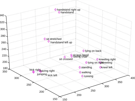
where x is a dataset sample, N the number of samples per set, and M the number of sets. This gives an indication how far apart the mean vectors of the contexts are located from each other. Figure 7 shows a mapping of all datasets2 and their means for the three most varying sensors amongst the thirty available (similar, but more straightforward than other linear mappings such as Principal Component Analysis or Independent Component Analysis), while Figure 9 depicts the resulting evaluation plot. The dispersion between the two datasets in Figure 8 for instance would be the sum of the squares of the distance from each cross to the mean of all crosses, divided by 2. Alternatively, variance or (semi) interquartile range can also be applied instead of standard variation.

0 5 10 15 20 25

30 0

5

10

15

20 0

5 10 15 20 25

# contexts # sensors

Figure 10. The 3D dispersion plot with the variance of the datasets incorporated.

The dispersion between weighted means adds the spread per dataset to the equation. The measure of dispersion is decreased for datasets that are spread over a wider area by weighting the means with the average standard deviation over all datasets. Entangled datasets such as the one in figure 8.2 will therefore become less dispersed, resulting in a more accurate measure. Figure 10 shows the plot with the dispersion between weighted means as the z-axis.

All context-datasets and Matlab scripts that were used to create these plots are available at:

http://www.comp.lancs.ac.uk/~kristof/notes/multi/

1

Sensor 1

2

Sensor 1

S

en

so

r

2

S

en

so

r

2

1

2

1

Many algorithms are based on either mean- or Gaussian-like modeling of the data, which leads to our assumption that this assessment is representative for a large number of classification algorithms.

3.4. Discussion

A first remark relates to the generalization of these particular plots: they are merely examples of how a context-aware algorithm would perform since they are primarily based on a basic (average- and variance based) modelling of each class. The dispersion measure is therefore not necessarily equal to recognition performance. The plots are furthermore highly dependent on both the chosen sensors and the contexts, so the plots should be viewed as a probe rather than a proof of a generic concept.

One immediate use for these kind of evaluation plots is that they show how specific sensors and contexts contribute to overall dispersion. It is for instance possible to inspect the plot for the largest increase of dispersion when a sensor is added to the system, or contexts that likewise decrease dispersion. Figure 10 shows for instance that in a system with many sensors (e.g. more than 10), dispersion will drop significantly if the last seven contexts are added. Such a decrease can also be noticed after the third, fourth and fifth context were added.

Both plots (see Figure 9 and 10) show that the sensor data enables most algorithms to perform better as the number of sensors increases. The slight glitches, where the performance for a set of contexts doesn’t increase monotonously as sensors are added, are caused by the selection procedure in which the sensors are sorted per added context based on their variance for the current set of contexts. Fluctuations in the contexts-axis appear occasionally for the same reason.

Another use for the latter plot is its indication on what we earlier called the complexity of the contexts: the more pattern-based contexts in our experiment, such as running, jumping, or kicking appear on the lower half of the plot of Figure 10 since their sensor readings are intertwined with each other and those of the other datasets. It is remarkable that these contexts do not perform better after adding more than two sensors. These same contexts appear early on in the first plot (Figure 9), as only the means are taken into account and variance is disregarded.

4.

Example of context -aware clothing

It is, as indicated by our experiments, feasible to distinguish certain activities of a wearer whose clothing

has an embedded distributed sensor network. These activities could also include gestures made by the user. Specifically more basic events related to garments, such as putting on a coat or taking off a coat, can be recognized with a reasonably high precision. This section briefly elaborates on such a feasible application where having a multitude of sensors and less (pre-) processing is an advantage that is hard to top by the existing traditional approaches.

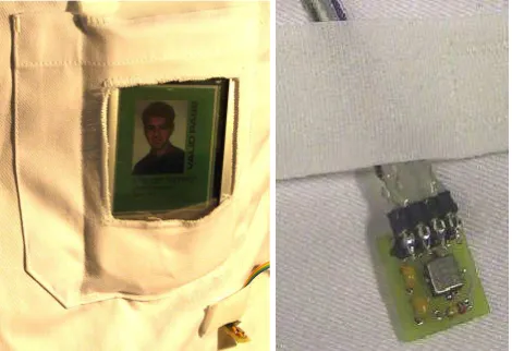
The prototype system consists of a lab coat with an embedded wearable computer, a dedicated authentication station, and a number of terminals for which access control is implemented. The lab coat is equipped with 14 accelerometers and holds an iPAQ in its front pocket (see Figure 11). The sensors are connected to the PIC-based I/O system which reads all the sensors and provides them on the serial line to the iPAQ, which also has access to the network using WLAN. The iPAQ calculates the worn/ not worn context, based on the sensor data, and communicates this to the authentication station for the initial setup and to the terminals for authentication. The iPAQ’s display is visible, similar to a name badge, to other people, showing the name and function of the user, a photo and whether or not the wearer is currently granted a valid pass.

Figure 11. The iPAQ (left), integrated in the front pocket of the lab coat, displays the current state, while (left) accelerometers across the lab coat sense the coat’s movement and position.

might apply this to speed up authentication or improve identification.

5.

Conclusions

Since multi-sensor wearable systems are relatively hard to realize, our knowledge of both recognition and added value of these systems is limited. Apart from the traditional centralized processing architecture of the sensor data, attention was given to truly distributed sensor processing as well, resulting in self-organization in a wireless sensor network. We aimed at extending our understanding by evaluating a multi-sensor system and analysing its data, under a variable number of sensors and targeted contexts. Experimenting with a large number of acceleration sensors distributed over the body, we found that performance can depend heavily on the number of sensors and contexts, but also on the nature of the contexts.

Furthermore, an application scenario was presented that takes advantage of the multitude of embedded acceleration sensors, to detect whether it is being worn. This is an attractive example, as designing this setup with fewer sensors would result in a less precise, and certainly less robust recognition of this context, regardless of the recognition algorithm.

Acknowledgements

This research was partially funded by the Equator IRC, EPSRC GR/N15986/01 (http://www.equator.ac.uk) and the Smart-Its project (sponsored by the Information Systems and Technology framework of the European Commission, http://www.smart-its.org ).

References

[1] G. Asada, M. Dong, T.S. Lin, F. Newberg, G. Pottie, W.J. Kaiser, and H.O. Marcy. “Wireless Integrated Network Sensors: Low Power Systems on a Chip.” Proceedings of the 1998 European Solid State Circuits Conference. 1998.

[2] R. R. Brooks. “Highly Redundant Sensing in Robotics – Analogies From Biology: Distributed Sensing and Learning”. In Proceedings of the NATO Advanced Research Workshop on Highly Redundant Sensing in Robotic Systems, Italy, 1988.

[3] P.J. Brown. “The stick-e Document: A Framework for creating context-aware Applications”. Proc. EP´96, Palo Alto, CA. (published in EP-odds, vol 8. No 2, pp. 259-72) 1996.

[4] E. Catterall, K. Van Laerhoven and M. Strohbach. “Self-Organization in Ad Hoc Sensor Networks: An Empirical

Study”. In Proc. of Alife VIII: the 8th International Conference on the Simulation and Synthesis of Living Systems, Sydney, Australia. MIT Press, 2002.

[5] A. Cerpa and D. Estrin. “Ascent: Adaptive Self-Configuring sEnsor Network Topologies” UCLA Computer Science Department Technical Report UCLA/CSD-TR-01-0009, May 2001.

[6] K. Cheverst G. Blair, N. Davies, and A. Friday. “Supporting Collaboration in Mobile-aware Groupware.” Personal Technologies, Vol 3, No 1, March 1999.

[7] R. Joshi & A. C. Sanderson. “Multi Sensor Fusion: A Minimal Representation Framework”. Series in Intelligent Control and Intelligent Automation - Vol. 11. SWPC.

[8] J. M. Kahn, R. H. Katz and K. S. J. Pister, "Mobile Networking for Smart Dust", ACM/IEEE Intl. Conf. on Mobile Computing and Networking (MobiCom 99), Seattle, WA, August 17-19, 1999.

[9] K. Kukkonen, T. Vuorela, J. Rantanen, O. Ryynänen, A. Siili, and J. Vanhala “The Design and Implementation of Electrically Heated Clothing.” In Proceedings of the Fifth International Symposium on Wearable Computers (ISWC’01), Zurich, 2001.

[10] A. Lim "Distributed Services for Information Dissemination in Self-Organizing Sensor Networks,", Special Issue on Distributed Sensor Networks for Real-Time Systems with Adaptive Reconfiguration, Journal of Franklin Institute, Elsevier Science Publisher, Vol. 338, 2001, pp. 707-727.

[11] F. Michahelles, M. Samulowitz and B. Schiele, “Detecting Context in Distributed Sensor Networks by Using Smart Context-Aware Packets”. In International Conference on Architecture of Computing Systems (ARCS) 2002, Karlsruhe, Germany, April 2002.

[12] A. Schmidt and K. Van Laerhoven. “How to build smart appliances”. In IEEE Personal Communications, Special Issue on Pervasive Computing, August 2001, Vol. 8, No. 4. pp. 66-71.

[13] The Smart-Its project: http://www.smart-its.org .

[14] T. Starner, B. Schiele, A. Pentland. “Visual Contextual Awareness in Wearable Computing”. Proceeding of the Second Int. Symposium on Wearable Computing. Pittsburgh, October 1998.