Localization induced coherent backscattering effect in wave dynamics

Localization-induced coherent backscattering effect in wave dynamics

H. Schomerus, K. J. H. van Bemmel, and C. W. J. Beenakker

Instituut-Lorentz, Universiteit Leiden, P.O. Box 9506, 2300 RA Leiden, The Netherlands 共Received 1 September 2000; published 22 January 2001兲

We investigate the statistics of single-mode delay times of waves reflected from a disordered waveguide in the presence of wave localization. The distribution of delay times is qualitatively different from the distribution in the diffusive regime, and sensitive to coherent backscattering: The probability of finding small delay times is enhanced by a factor close to

冑

2 for reflection angles near the angle of incidence. This dynamic effect of coherent backscattering disappears in the diffusive regime.

DOI: 10.1103/PhysRevE.63.026605 PACS number共s兲: 42.25.Dd, 42.25.Hz, 72.15.Rn

I. INTRODUCTION

The two most prominent interference effects arising from multiple scattering are coherent backscattering and wave lo-calization 关1–6兴. Both effects are related to the static inten-sity of a wave reflected or transmitted by a medium with randomly located scatterers. Coherent backscattering is the enhancement of the reflected intensity in a narrow cone around the angle of incidence, and is a result of the system-atic constructive interference in the presence of time-reversal symmetry关4,5兴. Localization arises from systematic destruc-tive interference, and suppresses the transmitted intensity关6兴. This paper presents a detailed theory of a recently discov-ered关7兴interplay between coherent backscattering and local-ization in a dynamic scattering property, the single-mode de-lay time of a wave reflected by a disordered waveguide. The single-mode delay time is the derivative ␾

⬘

⫽d␾/d␻ of the phase␾of the wave amplitude with respect to the frequency ␻. It is linearly related to the Wigner-Smith delay times of scattering theory关8–10兴, and is the key observable of recent experiments on multiple scattering of microwaves 关11兴 and light waves 关12兴. Van Tiggelen, et al.关13兴developed a sta-tistical theory for the distribution of ␾

⬘

in a waveguide ge-ometry共where angles of incidence are discretized as modes兲. Although the theory was worked out mainly for the case of transmission, the implications for reflection are that the dis-tribution P(␾

⬘

) does not depend on whether the detected mode n is the same as the incident mode m or not. Hence it appears that no coherent backscattering effect exists for P(␾

⬘

).

What we will demonstrate here is that this is true only if wave localization may be disregarded. Previous studies 关11,13兴dealt with the diffusive regime of waveguide lengths L below the localization length␰.共The localization length in a waveguide geometry is ␰⯝Nl, with N the number of propagating modes and l the mean free path.兲Here we con-sider the localized regime L⬎␰ 共assuming that also the ab-sorption length␰a⬎␰). The distribution of reflected intensity

is insensitive to the presence or absence of localization, be-ing given in both regimes by Rayleigh’s law. In contrast, we find that the delay-time distribution changes markedly as one enters the localized regime, decaying more slowly for large 兩␾

⬘

兩. Moreover, a coherent backscattering effect appears: For L⬎␰ the peak of P(␾

⬘

) is higher for n⫽m than for n

⫽m by a factor which is close to

冑

2, the precise factor being

冑

2⫻(4096/1371␲)⫽1.35.

We also consider what happens if time-reversal symmetry is broken, by some magneto-optical effect. The coherent backscattering effect disappears. However, even for n⫽m, the delay-time distribution for preserved time-reversal sym-metry is different than for broken time-reversal symsym-metry. This difference is again only present for L⬎␰, and vanishes in the diffusive regime.

The plan of this paper is as follows: In Sec. II we specify the notion关11兴of the single-mode delay time␾

⬘

, relate it to the Wigner-Smith delay times, and review the results 关13兴 for the diffusive regime, extending them to include ballistic corrections. This section also contains the random-matrix formulation for the localized regime, that provides the basis for our calculations, and includes a brief discussion of the conventional coherent backscattering effect in the static in-tensity I. Section III presents the calculation of the joint dis-tribution of␾

⬘

and I. We compare our analytical theory with numerical simulations, and give a qualitative argument for the dynamic coherent backscattering effect. The role of ab-sorption is discussed, as well as the effect of broken time-reversal symmetry. Details of the calculation are delegated to the Appendixes.

II. DELAY TIMES A. Single-mode delay times

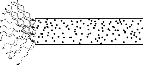
We consider a disordered medium共mean free path l) in a waveguide geometry共length L), as depicted in Fig. 1. There are NⰇ1 propagating modes at frequency ␻, given by N ⫽␲A/␭2 for a waveguide with an opening of areaA. The wave velocity is c, and we consider a scalar wave共 disregard-ing polarization兲for simplicity. In the numerical simulations we will work with a two-dimensional waveguide of width W, where N⫽2W/␭.

We study the dependence of the reflected wave amplitude

rnm⫽

冑

Iei␾ 共1兲

on the frequency␻. The indices n and m specify the detected and incident mode, respectively. 共We assume single-mode excitation and detection.兲 Here I⫽兩rnm兩2 is the intensity of

intensity, and characterizes the static properties of the re-flected wave. Dynamic information is contained in the phase derivative

␾

⬘

⫽d␾

d␻, 共2兲

which has the dimension of a time and is called the single-mode delay time 关11,13兴. The intensity I and the delay time ␾

⬘

can be recovered from the product of reflection matrix elements

␳⫽rnm共␻⫹

1

2␦␻兲rnm* 共␻⫺

1

2␦␻兲, 共3兲

evaluated at two nearby frequencies ␻⫾12␦␻. To leading

order in the frequency difference␦␻ one has

␳⫽I共1⫹i␦␻␾

⬘

兲⇒I⫽ lim ␦␻→0

Re␳, ␾

⬘

⫽ lim ␦␻→0

Im␳ ␦␻I.

共4兲

We seek the joint distribution function P(I,␾

⬘

) in an en-semble of different realizations of disorder. We distinguish between the diffusive regime where L is small compared to the localization length ␰⯝Nl, and the localized regime where Lⲏ␰. Localization also requires that the absorption length ␰aⲏ␰. We will contrast the case of excitation and

detection in two distinct modes n⫽m with the equal-mode case n⫽m. Although we mainly focus on the optically more relevant case of preserved time-reversal symmetry, we will also discuss the case of broken time-reversal symmetry for comparison. These two cases are indicated by the indexes ␤⫽1 and 2, respectively.

B. Relation to Wigner-Smith delay times

In the localized regime (␰ⰆL,␰a) we can relate the

single-mode delay time ␾

⬘

to the Wigner-Smith关8–10兴 de-lay times ␶i, with i⫽1, . . . ,N. The ␶i’s are defined for a

unitary reflection matrix r 共composed of the elements rnm);

hence they require the absence of transmission and of ab-sorption. One then has

⫺ir†dr d␻⫽U

† _{diag共␶1, . . . ,␶}

N兲U, 共5a兲

⫺ir*dr T

d␻⫽V

† _{diag共␶1, . . . ,␶}

N兲V, 共5b兲

with U and V unitary matrices of eigenvectors. In the pres-ence of time-reversal symmetry r is a symmetric matrix; hence V⫽U in this case.

For small ␦␻we can expand

r共␻⫾1

2␦␻兲⫽V

T_U⫾1 2i␦␻V

T _{diag共␶1, . . . ,␶}

N兲U. 共6兲

Inserting this into Eq. 共3兲and comparing with Eq.共4兲yields the relations

␾

⬘

⫽ReA1 A0

, I⫽兩A0兩2, A_k⫽

兺

i ␶i

k_u

ivi. 共7兲

We have abbreviated ui⫽Uim and vi⫽Vin. In the special

case n⫽m, the coefficients ui and vi are identical in the

presence of time-reversal symmetry.

The distribution of the Wigner-Smith delay times in the localized regime was determined recently 关14兴. In terms of the rates ␮i⫽1/␶i it has the form of the Laguerre ensemble

of random-matrix theory,

P共兵␮i其兲⬀

兿

i⬍j 兩␮i⫺␮j兩 ␤

兿

k ⌰共␮k兲

e⫺␥(␤N⫹2⫺␤)␮k_, 共₈兲

where the step function ⌰(x)⫽1 for x⬎0 and 0 for x⬍0. The parameter ␥ is defined by

␥⫽␣l/c, 共9兲

with the coefficient ␣⫽␲2_{/4 or 8/3 for two- or} three-dimensional scattering, respectively. Equation 共8兲 extends the N⫽1 result of Refs.关15–17兴to any N.

The matrices U and V in Eq.共6兲are uniformly distributed in the unitary group. They are independent for ␤⫽2, while U⫽V for ␤⫽1. In the large-N limit the matrix elements become independent Gaussian random numbers with vanish-ing mean and variance 1/N. Hence

具

ui

典

⫽

具

vi

典

⫽0,

具兩

ui兩2

典

⫽

具

兩vi兩2

典

⫽N⫺1, 共10兲

with u_i⫽vifor n⫽m and␤⫽1. Corrections to this Gaussian

approximation are of order 1/N.

C. Diffusion theory

The joint probability distribution P(I,␾

⬘

) in the diffusive regime lⰆLⰆ␰ was derived in Refs.关11,13兴,

Pdiff共I,␾

⬘

兲⫽⌰共I兲共I/␲¯I3兲1/2e⫺I/ I

¯

共Q␾¯

⬘

2兲⫺1/2

⫻exp

冉

⫺I I ¯

共␾

⬘

⫺␾¯

_⬘

_兲2

[image:2.612.57.296.61.170.2]

Q␾¯

⬘

2

冊

, 共11兲

with constants I¯, ␾¯

⬘

, and Q. It has the same form for trans-mission and reflection, the only difference being the depen-dence of the constants on the system parameters. Here we focus on the case of reflection, because we are concerned with coherent backscattering.

From the joint distribution function 关Eq. 共11兲兴, for the intensity one obtains the Rayleigh distribution

Pdiff共I兲⫽ 1 I

¯exp共⫺I/ I¯兲. 共12兲

Hence I¯ is the mean detected intensity per mode. It is given by关18兴

I ¯_⫽1

N共1⫹␦␤1␦nm兲, 共13兲

assuming unit incident intensity. The factor of 2 enhance-ment in the case n⫽m is the static coherent backscattering effect mentioned in Sec. I, which exists only in the presence of time-reversal symmetry (␤⫽1). Equations共12兲and共13兲 remain valid in the localized regime, since they are deter-mined by scattering on the scale of the mean free path. Hence LⰇl is sufficient for static coherent backscattering, and it does not matter whether L is small or large compared to␰.

By integrating over I in Eq.共11兲one arrives at the distri-bution of single-mode delay times关11,13兴,

Pdiff共␾

⬘

兲⫽ Q

2␾¯

⬘

关Q⫹共␾

⬘

/␾

¯

_⬘

_⫺1兲2_兴⫺3/2_{. 共14兲}

Hence␾¯

⬘

is the mean delay time, while

冑

Q sets the relative width of the distribution. These constants are determined by the correlator 关11,13兴

C12⫽

具

rnm共␻⫹␦␻兲rnm* 共␻兲

典

具

rnm共␻兲rnm* 共␻兲

典

⫽1⫹i␾¯

⬘

␦␻⫺1

2␾¯

⬘

2_{共Q⫹1兲共␦␻兲}2_{. 共15兲}

Diffusion theory gives

␾

¯

_⬘

_{⫽2␥s/3, Q⫽2s/5. 共16兲}

Here␥ is given by Eq.共9兲. We have defined

s⫽␣

⬘

L/l, 共17兲

where the numerical coefficient ␣

⬘

⫽2/␲, 3/4 for two- and three-dimensional scattering.共The corresponding result for Q given in Ref. 关13兴is incorrect.兲

Diffusion theory predicts that the distribution of delay times 关Eq. 共14兲兴, as well as the values of the constants ␾¯

⬘

and Q, do not depend on the choice n⫽m or n⫽m 共and also not on whether time-reversal symmetry is preserved or not兲. Hence there is no dynamic effect of coherent backscattering in the diffusive regime.

D. Ballistic corrections

The expressions for the constants I¯, ␾¯

⬘

, and Q given above are valid up to corrections of order l/L. Here we give more accurate formulas that account for these ballistic cor-rections.共We need these to compare with numerical simula-tions.兲 We determine the ballistic corrections for Q and␾¯

⬘

by relating the dynamic problem to a static problem with absorption. 共This relationship only works for the mean. It cannot be used to obtain the distribution 关19兴.兲 The mean total reflectivity

a

¯_⫽1⫹x⫺

冑

_2x⫹x2_coth关s

冑

_2x⫹x2_{⫹arcosh共1⫹x兲兴} 共18兲

for absorption␣

⬘

x per mean free path was evaluated in Ref. 关20兴.关Here␣

⬘

is the same constant as in the definition of s; see Eq. 共17兲.兴 We identify C12⫽¯ (x)/a¯(0) by analyticala continuation to an imaginary absorption rate x⫽⫺i␦␻␥. Expanding in x to second order, we find

␾

¯

_⬘

_⫽␥s共3⫹2s兲 3共1⫹s兲 , Q⫽

8s3⫹28s2⫹30s⫹15 5共2s⫹3兲2 . 共19兲

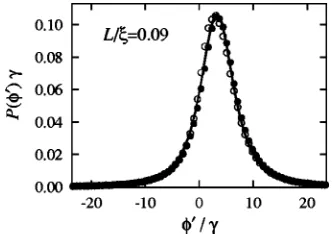
E. Numerical simulation

The validity of diffusion theory was tested in Refs.关11– 13兴by comparison with experiments in transmission. In Fig. 2 we show an alternative test in reflection, by comparison with a numerical simulation of scattering of a scalar wave by a two-dimensional random medium. 共We assume time-reversal symmetry.兲The reflection matrices r(␻⫾1

2␦␻) are

computed by applying the method of recursive Green func-tions关21兴to the Helmholtz equation on a square lattice共 lat-tice constant a). The width W⫽100 a and the frequency␻ ⫽1.4 c/a are chosen such that there are N⫽50 propagating modes. The mean free path l⫽14.0 a is found from the for-mula关22兴tr rr†_⫽Ns(1⫹s)⫺1 _{for the reflection probability.} The corresponding localization length ␰⫽NL/s⫽1100 a. The parameter␥⫽46.3 a/c is found from Eq.共19兲by

equat-FIG. 2. Distribution of the single-mode delay time ␾⬘ in the diffusive regime. The result of numerical simulation 共data points兲 with N⫽50 propagating modes is compared to the prediction关Eq.

共14兲兴 of diffusion theory共solid curve兲. There is no difference be-tween the case n⫽m of equal-mode excitation and detection共open circles兲 and the case n⫽m of excitation and detection in distinct

[image:3.612.354.520.57.174.2]

ing

具

␾

⬘

典

⫽␾¯

⬘

.共This value of␥ is somewhat larger than the value ␥⫽␲2l/4c⫽34.5 a/c expected for two-dimensional scattering, as a consequence of the anisotropic dispersion relation on a square lattice.兲 We will use the same set of parameters later in this paper in the interpretation of the re-sults in the localized regime. Our numerical rere-sults confirm that in the diffusive regime the distribution of delay times␾

⬘

does not distinguish between excitation and detection in dis-tinct modes (n⫽m, full circles兲and identical modes (n⫽m, open circles兲.

III. DYNAMIC COHERENT BACKSCATTERING EFFECT A. Distinct-mode excitation and detection

We now calculate the joint probability distribution func-tion P(I,␾

⬘

) of intensity I and single-mode delay time␾

⬘

in the localized regime, for the typical case n⫽m of excitation and detection in two distinct modes. We assume a preserved time-reversal symmetry (␤⫽1), leaving the case of broken time-reversal symmetry for the end of this section.

It is convenient to work momentarily with the weighted delay time W⫽␾

⬘

I and to recover P(I,␾

⬘

) from P(I,W) at the end. The characteristic function

␹共p,q兲⫽

具

e⫺i pI⫺iqW

典

共20兲

is the Fourier transform of P(I,W). The average

具

•••

典

is over the vectors u and v and over the set of eigenvalues兵␶i其.

The average over one of the vectors, say v, is easily carried out, because it is a Gaussian integration. The result is a de-terminant:

␹共p,q兲⫽

具

det共1⫹iH/N兲⫺1

典

, 共21a兲

H⫽pu*uT⫹1 2q共u¯*u

T_⫹u*¯uT_{兲. 共21b兲}

The Hermitian matrix H is a sum of dyadic products of the vectors u and u¯, with u¯_i⫽u_i␶_i, and hence has only two non-vanishing eigenvalues ␭_⫹ and ␭_⫺. Some straightfor-ward linear algebra gives

␭_⫾⫽1

2共qB1⫹p⫾

冑

2 pqB1⫹q2B2⫹p2兲, 共22兲 where we have defined the spectral moments

Bk⫽

兺

i 兩

ui兩2␶i

k_{. 共23兲}

The resulting determinant is

det共1⫹H/N兲⫺1⫽共1⫹␭_⫹/N兲⫺1共1⫹␭_⫺/N兲⫺1; 共24兲

hence

␹共p,q兲⫽

冓

冋

1⫹i p N⫹

iq

NB1⫹ q2

4N2共B2⫺B1 2_兲

册

⫺1

冔

. 共25兲

An inverse Fourier transform, followed by a change of vari-ables from I,W to I,␾

⬘

, gives

P共I,␾

⬘

兲⫽⌰共I兲共N3I/␲兲1/2e⫺NI

⫻

冓

共B2⫺B1

2_兲⫺1/2_exp

冉

_⫺NI共␾

⬘

⫺B1兲 2

B2⫺B1 2

冊

冔

.

共26兲

The average is over the spectral moments B1 and B2, which depend on the u_i’s and ␶_i’s via Eq. 共23兲.

The calculation of the joint distribution P(B1,B2) is pre-sented in Appendix A. The result is

P共B1,B2兲⫽⌰共B1兲⌰共B2兲exp

冉

⫺ NB₁2

B2

冊

⫻

冋

B1 2

␥N3

B₂4 共B2⫹␥N 2_B

1兲exp

冉

⫺ 2␥N

B1

冊

⫺␥ 3_N5

4B₂5 共2B2 2_⫺4B

1 2_B

2N⫹B1

4_N2_兲Ei

冉

_⫺2␥N B1

冊

册

,

共27兲

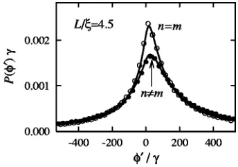
where Ei(x) is the exponential-integral function. The distri-bution P(I,␾

⬘

) follows from Eq.共26兲by integrating over B1 and B2 with weight given by Eq.共27兲.

Irrespective of the distribution of B1 and B2, from Eq. 共26兲we recover the Rayleigh law关Eq.共12兲兴for the intensity I. The distribution P(␾

⬘

)⫽兰₀⬁d I P(I,␾

⬘

) of the single-mode delay time takes the form

P共␾

⬘

兲⫽

冕

0

⬁ dB1

冕

0

⬁ dB2

P共B1,B2兲共B2⫺B1 2_兲

2共B2⫹␾

⬘

2⫺2B1␾

⬘

兲3/2 . 共28兲

[image:4.612.351.523.57.178.2]

In Fig. 3 this distribution is compared with the result of a numerical simulation of a random medium as in Sec. II E, but now in the localized regime. The same value for ␥ was used as in Fig. 2, making this comparison a parameter-free test of the theory.共Note that␥alone determines the complete distribution function in the localized regime, in contrast to

FIG. 3. Distribution of the single-mode delay time ␾⬘ in the localized regime. The results of numerical simulations with N

⫽50 propagating modes共open circles for n⫽m, full circles for n

⫽m) are compared to the analytical predictions. The curve for

the diffusive case where two parameters are required.兲The numerical data agree very well with the analytical prediction.

B. Equal-mode excitation and detection

We now turn to the case n⫽m of equal-mode excitation and detection, still assuming that time-reversal symmetry is preserved. Since ui⫽vi, we now have

␾

⬘

⫽ReC1 C0

, I⫽兩C0兩2, Ck⫽

兺

i ␶i

k_u i

2_{. 共29兲}

The joint distribution function P(C0,C1) of these complex numbers can be calculated in the same way as P(B1,B2). In Appendix C we obtain

P共C0,C1兲⬀exp共⫺N兩C0兩2/2兲

冕

0

⬁

dss2e⫺s

⫻

冉

1⫹兩C1兩 2_s2

␥2_N2 ⫺ 2s

␥NRe C0C1*

冊

⫺5/2 . 共30兲

The corresponding distribution function P(␾

⬘

) is also plot-ted in Fig. 3, and compared with the results of the numerical simulation. Good agreement is obtained, without any free parameter.

C. Comparison of both situations

Comparing the two curves in Fig. 3, we find a striking difference between distinct-mode and equal-mode excitation and detection: The distribution for n⫽m displays an en-hanced probability of small delay times. In the vicinity of the peak, both distributions become very similar when the delay times for n⫽m are divided by a scale factor of about

冑

2. In the limit N→⬁ 共see Sec. III D兲, the maximal value P(␾peak

⬘

)⫽

冑

2/␲N3␥2 for n⫽m is larger than the maximum of P(␾

⬘

) for n⫽m by a factor

Pn_⫽m共␾peak

⬘

兲

Pn⫽m共␾peak

⬘

兲

⫽

冑

2⫻ 4096

1371␲⫽1.35. 共31兲

Correspondingly, the probability to find very large delay times is reduced for n⫽m. This is reflected by the asymptotic behavior

P共␾

⬘

兲⬃␥N 3/2

␾

⬘

2

再

共2␲兲⫺1/2 for n⫽m

冑␲

/4 for n⫽m. 共32兲

The enhanced probability of small delay times for n⫽m is the dynamic coherent backscattering effect mentioned in Sec. I. The effect requires localization, and is not observed in the diffusive regime.

D. Limit N\ⴥ

The results presented so far assume NⰇ1, but retain finite-N corrections of order N⫺1/2.共Only terms of order 1/N and higher are neglected.兲It turns out that the asymmetry of

P(␾

⬘

) for positive and negative values of␾

⬘

is an effect of order N⫺1/2. The asymmetry is hence captured faithfully by our calculation. We now consider how the asymmetry even-tually disappears in the limit N→⬁.

For distinct modes n⫽m, the spectral moments scale as B1⬃␥N and B2⬃␥2N3. With␾

⬘

⬃␥N3/2, one finds that B1 can be omitted to order N⫺1/2 in Eq.共28兲. One obtains the symmetric distribution

P共␾

⬘

兲⫽

冕

0

⬁ dB2

P共B₂兲B₂

2共B₂⫹␾

⬘

2_兲3/2 共33兲

plotted in Fig. 4.

For identical modes n⫽m, observe that the quantities C0 and C₁ become mutually independent in the large-N limit: The cross-term (␥N)⫺1 Re C0C1* in Eq. 共30兲 is of relative order N⫺1/2 because C0⬃N⫺1/2 and C1⬃␥N. Hence, to or-der N⫺1/2, the distribution factorizes, P(C0,C1) ⫽P(C₀) P(C₁). The distribution of C₀ is a Gaussian,

P共C₀兲⫽ N

2␲exp共⫺N兩C0兩

2_{/2兲, 共34兲}

as a consequence of the central-limit theorem, and

P共C1兲⬀

冕

0

⬁

dss2e⫺s

冉

1⫹兩C1兩 2_s2

␥2_N2

冊

⫺5/2

. 共35兲

The resulting distribution of ␾

⬘

⫽Re(C1/C0) is also plotted in Fig. 4.

[image:5.612.356.522.56.176.2]

The dynamic coherent backscattering effect persists in the limit N→⬁, it is therefore not due to finite-N corrections. The peak heights differ by the factor given in Eq. 共31兲.

FIG. 4. Distribution of the single-mode delay time ␾⬘ in the localized regime for preserved time-reversal symmetry, in the limit

E. Interpretation in terms of large fluctuations In order to explain the coherent backscattering enhance-ment of the peak of P(␾

⬘

) in more qualitative terms, we compare Eq. 共29兲for n⫽m with the corresponding relation 关Eq. 共7兲兴for n⫽m.

The factorization of the joint distribution function P(C0,C1) discussed in Sec. III D can be seen as a conse-quence of the high density of anomalously large Wigner-Smith delay times␶iin the Laguerre ensemble关Eq.共8兲兴. The

distribution of the largest time␶max⫽maxi␶ifollows from the

distribution of the smallest eigenvalue in the Laguerre en-semble, calculated by Edelman关23兴. It is given by

P共␶max兲⫽␥N 2

␶max2 exp共⫺␥N

2_{/␶max兲. 共36兲}

As a consequence, the spectral moment C₁is dominated by a small number of contributions u_i2␶i共often enough by a single

one, say with index i⫽1), while C0 can be safely approxi-mated by the sum over all remaining indices i 共say, i⫽1). The same argument applies also to the spectral moments Ak

which determine the delay-time statistics for n⫽m; hence the distribution function P(A₀,A₁) factorizes as well.

The quantities A0 and C0have a Gaussian distribution for large N, because of the central-limit theorem, with P(C₀) given by Eq.共34兲and

P共A₀兲⫽N

␲exp共⫺N兩A0兩2兲. 共37兲

It then becomes clear that the main contribution to the en-hancement关Eq. 共31兲兴of the peak height, namely, the factor of

冑

2, has the same origin as the factor of 2 enhancement of the mean intensity I¯. More precisely, the relation P(A0⫽x) ⫽2 P(C0⫽

冑

2x) leads to a rescaling of P(I) for n⫽m by a factor of 1/2 and to a rescaling of P(␾

⬘

) by a factor of

冑

2. The remaining factor of 4096/1371␲⫽0.95 comes from the difference in the distributions P(A₁) and P(C₁). It turns out that the distribution

P共A₁兲⫽

冕

0

⬁ ds 1

4␲␥N

s2

共4⫹兩A1/␥N兩2s2兲3

⫻关e⫺s共64⫹32s⫹12s2⫹s3兲⫺3s2 Ei共⫺s兲兴 共38兲

共derived in Appendix D兲is very similar to P(C₁) given in Eq. 共35兲; hence the remaining factor is close to unity.

The large ␶i’s are related to the penetration of the wave

deep into the localized regions and are eliminated in the dif-fusive regime Lⱗ␰. In Sec. III F we compare the localized and diffusive regimes in more detail.

F. Localized vs diffusive regime

Comparison of Eqs.共11兲and共26兲shows that the two joint distributions of I and␾

⬘

would be identical if statistical fluc-tuations in the spectral moments B₁and B₂could be ignored. The correspondences are

B1↔␾¯

⬘

, B2⫺B1

2_↔Q␾¯

_⬘

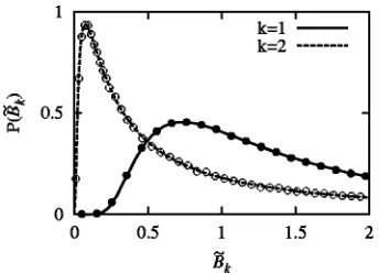
2_{. 共39兲}

However, the distribution P(B1,B2) is very broad 共see Fig. 5兲, so that fluctuations cannot be ignored. The most probable values are

B₁typical⯝␥N, B₂typical⯝␥2N3, 共40兲

but the mean values

具

B1典,

具

B2典 diverge—demonstrating the presence of large fluctuations. In the diffusive regime Lⱗ␰ the spectral moments B1 and B2 can be replaced by their ensemble averages, and the diffusion theory关11,13兴is recov-ered. 共The same applies if the absorption length␰_aⱗ␰.兲

The large fluctuations in B1 and B2 directly affect the statistical properties of the delay time ␾

⬘

. We compare the distribution 关Eq. 共28兲兴 in the localized regime 共Fig. 3兲 with the result关Eq.共14兲兴of diffusion theory共Fig. 2兲. In the local-ized regime the value␾peak

⬘

⯝B₁typicalat the center of the peak of P(␾

⬘

) is much smaller than the width of the peak⌬␾

⬘

⯝(B₂typical)1/2⯝␾_peak

⬘

(␰/l)1/2. This also holds in the diffusive regime, where␾peak

⬘

⫽␾¯

⬘

and⌬␾

⬘

⯝␾peak

⬘

(L/l)1/2_{. However,} the mean

具␾

⬘

典

⫽

具

B1典 diverges for P, but is finite共equal to ␾¯

_⬘

_{) for Pdiff. For large B2 one has, asymptotically, P(B2)} ⬃1

4N␥

3/2

冑␲

_B 2

⫺3/2

. As a consequence, in the tails P(␾

⬘

) falls off only quadratically关see Eq.共32兲兴, while in the diffu-sive regime Pdiff(␾

⬘

)⬃

1 2Q␾¯

⬘

2_兩␾

_⬘

_兩⫺3 _{falls off with an} in-verse third power.

G. Role of absorption

[image:6.612.352.524.56.180.2]

Although absorption causes the same exponential decay of the transmitted intensity as localization, this decay is of a quite different, namely, an incoherent, nature. The strong fluctuations in the localized regime disappear as soon as the absorption length ␰_a drops below the localization length␰, because long paths which penetrate into the localized regions

FIG. 5. Distributions of B˜1⫽B1/␥N and B˜2⫽B2/␥2N3. The

analytic prediction from Eq. 共27兲 关for explicit formulas see Eqs.

are suppressed by absorption. In this situation one should expect that the results of diffusion theory are again valid even for Lⲏ␰. This expectation is confirmed by our numeri-cal simulations.共We do not know how to incorporate absorp-tion effects into our analytical theory.兲

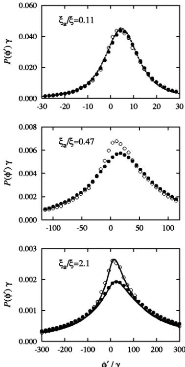
In Fig. 6 we plot the delay-time distribution for two val-ues of the absorption length␰a⬍␰and one value␰a⬎␰, both

for equal-mode and distinct-mode excitation and detection. The length of the waveguide is L⫽4.1␰. The result for strong absorption with ␰a⫽0.11␰ is very similar to Fig. 2.

Irrespective of the choice of the detection mode, the data can be fitted to prediction 共14兲of diffusion theory. The plot for ␰a⫽0.47␰ shows that the dynamic coherent backscattering

effect slowly sets in when the absorption length becomes comparable to the localization length. The data also deviate from the prediction of diffusion theory. The full factor关Eq. 共31兲兴 between the peak heights quickly develops as soon as

␰a exceeds ␰, as can be seen from the data for ␰a⫽2.1␰.

Moreover, these data can already be fitted to the predictions of random-matrix theory, with ␥⬇53.2 a/c. 共The value ␥ ⫽46.3 a/c of Sec. II E is reached when absorption is further reduced.兲

H. Broken time-reversal symmetry

The case ␤⫽2 of broken time-reversal symmetry is less important for optical applications, but has been realized in microwave experiments关24–26兴. There is now no difference between n⫽m and n⫽m. The matrices U and V have the same statistical distribution as for the case of preserved time-reversal symmetry. Hence, by following the steps of Sec. III A, we arrive again at Eq. 共26兲, with spectral moments Bk

as defined in Eq.共23兲. Their joint distribution has now to be calculated from Eq.共8兲with␤⫽2. This calculation is carried out in Appendix B. The result is

P共B₁,B₂兲⫽2␥N 3_B

1 2

B₂3 exp共⫺NB1 2_/B

2⫺2␥N/B1兲. 共41兲

The distribution of single-mode delay times P(␾

⬘

) is given by Eq.共28兲, with the function P(B1,B2). We plot P(␾

⬘

) in Fig. 7, and compare it to the case of preserved time-reversal symmetry. The distribution is rescaled by about a factor of 2 toward larger delay times when time-reversal symmetry is broken. This can be understood from the fact that the rel-evant length scale, the localization length, is twice as large for broken time-reversal symmetry (␰⫽2NL/s, while ␰ ⫽NL/s for preserved time-reversal symmetry兲.

IV. CONCLUSION

[image:7.612.78.267.56.430.2]

We have presented a detailed theory, supported by nu-merical simulations, of a recently discovered 关7兴 coherent backscattering effect in the single-mode delay times of a wave reflected by a disordered waveguide. This dynamic ef-fect is special because it requires localization for its exis-tence, in contrast to the static coherent backscattering effect in the reflected intensity. The dynamic effect can be under-stood from the combination of the static effect and the large

FIG. 6. Single-mode delay-time distribution P(␾⬘) in the pres-ence of absorption. The data points are the result of a numerical simulation of a waveguide with length L⫽4.5␰. Open circles are for equal-mode excitation and detection n⫽m, and full circles for the

case of distinct modes n⫽m. In the upper panel 共with␰a⬍␰), the

data are compared to the prediction关Eq.共14兲兴of diffusion theory. In the lower panel we compare with the predictions 关Eqs. 共27兲–

[image:7.612.355.521.56.178.2]

共30兲兴of random-matrix theory.

FIG. 7. Comparison of the single-mode delay-time distributions for preserved and broken time-reversal symmetry. The number of propagating modes is N⫽50. The curves are calculated from Eq.

共28兲, with P(B1,B2) given by Eq. 共27兲 (␤⫽1) or Eq. 共41兲 (␤

fluctuations in the localized regime.

In the diffusive regime there is no dynamic coherent backscattering effect: The distribution of delay times is un-affected by the choice of the detection mode and the pres-ence or abspres-ence of time-reversal symmetry. The effect also disappears when the absorption length is smaller than the localization length. In both situations the large fluctuations characteristic of the localized regime are suppressed.

Existing experiments on the delay-time distribution 关11,12兴verified the diffusion theory关13兴. The theory for the localized regime presented here awaits experimental verifi-cation.

ACKNOWLEDGMENTS

We thank P. W. Brouwer for valuable advice. This work was supported by the ‘‘Nederlandse organisatie voor Weten-schappelijk Onderzoek’’共NWO兲and by the ‘‘Stichting voor Fundamenteel Onderzoek der Materie’’共FOM兲.

APPENDIX A: JOINT DISTRIBUTION OF B1AND B2FOR␤Ä1

We calculate the joint probability distribution function P(B1,B2) of the spectral moments B1and B2, defined in Eq. 共23兲, which determine P(I,␾

⬘

) from Eq. 共26兲. We assume preserved time-reversal symmetry (␤⫽1). Since Bk ⫽兺i兩ui兩2␮i⫺

k

, we have to average over the wave function amplitudes ui, which are Gaussian complex numbers with

zero mean and variance 1/N, and the rates ␮i which are

distributed according to the Laguerre ensemble关Eq.共8兲兴with ␤⫽1. This Laguerre ensemble is represented as the eigen-values of an N⫻N Hermitian matrix W†W, where W is a complex symmetric matrix with the Gaussian distribution:

P共W兲⬀exp关⫺␥共N⫹1兲tr W†W兴. 共A1兲

The calculation is performed neglecting corrections of order 1/N, so that we are allowed to replace N⫹1 by N. The mea-sure is

dW⫽

兿

i_⬍j

d Re Wi jd Im Wi j

兿

i

d Re Wiid Im Wii. 共A2兲

1. Characteristic function

In the first step we express P(B1,B2) by its characteristic function,

P共B1,B2兲⫽ 1 共2␲兲2

冕

⫺⬁

⬁ d p

冕

⫺⬁ ⬁

dqei pB1⫹iqB2␹共_p,q兲_,

共A3兲

␹共p,q兲⫽

冓

兿

l_⫽1

N

exp

冋

⫺i兩ul兩2

冉

p ␮l

⫹ q

␮l

2

冊

册

冔

, 共A4兲 and average over the u_l’s:

␹共p,q兲⫽

冓

兿

l⫽1

N

冉

1⫹i p ␮lN⫹

i q ␮l

2_N

冊

⫺1

冔

⫽

冓

det共W

†_W兲2

det关共W†W兲2⫹i p共W†W兲/N⫹iq/N兴

冔

. 共A5兲

We have expressed the product over eigenvalues as a ratio of determinants. We write the determinant in the denominator as an integral over a complex vector z:

␹共p,q兲⬀

冕

dW

冕

dz exp关⫺␥N tr W†W兴det共W†W兲2 ⫻exp兵⫺z†关共W†W兲2⫹i p共W†W兲/N⫹iq/N兴z其.

共A6兲

This integral converges because W†W is positive definite.

2. Parametrization of the matrix W

Now we choose a parametrization of W which facilitates a stepwise integration over its degrees of freedom. The distri-bution of W is invariant under transformations W→UTWU, with any unitary matrix U. Hence we can choose a basis in which z points in direction 1, and write W in block form:

W⫽

冉

a xT

x X

冊

. 共A7兲

Here a is a complex number. For any (N⫺1)-dimensional vector x we can use another unitary transformation on the X block after which x points in direction 2. Then W is of the form

W⫽

冉

a x 0T x b yT

0 y Y

冊

, 共A8兲

with the real number x⫽兩x兩. In this parametrization

共W†_W兲

11⫽兩a兩2⫹x2, 关共W†_W兲2_兴

11⫽共兩a兩2⫹x2兲2⫹x2y2⫹x2兩a⫹b*兩2, det W⫽关a共b⫺yT_Y⫺1_y兲⫺x2_{兴det Y ,}

tr W†_W⫽兩a兩2_⫹兩b兩2_⫹2x2_⫹2y2_{⫹tr Y ,}

d W⫽d2_{a d}2_{bdx dy dY ,}

with y⫽兩y兩. A suitable transformation on Y allows one to replace the term yT_Y⫺1_{y by y}2_(Y⫺1₎

11.

For this parametrization of W, the integrand in Eq. 共A6兲 depends on the vectors x, y, and z only by their magnitudes x, y, and z⫽兩z兩. Hence we can replace dx→x2N⫺3dx, dy

3. Integration

The integrand in Eq.共A6兲involves z, p, and q in the form

exp†⫺z2共关共W†W兲2兴11⫹i p共W†W兲11/N⫹iq/N兲‡. 共A9兲

It is convenient to pass back to P(B₁,B₂) by Eq.共A3兲, be-cause integration over p and q gives delta functions: ␦关B1⫺z2共兩a兩2⫹x2兲/N兴␦共B2⫺z2/N兲

⫽_B1 2␦共

B1/B2⫺兩a兩2⫺x2兲␦共B2⫺z2/N兲. 共A10兲

Subsequent integration over z results in

P共B1,B2兲⬀

冕

d2ad2bdxdy x2N⫺3y2N⫺5B2

N⫺2_␦

⫻共B1/B2⫺兩a兩2⫺x2兲关c0

⫻兩ab⫺x2兩4⫹4c2兩a兩2y4兩ab⫺x2兩2⫹c4兩a兩4y8兴

⫻exp

冋

⫺NB₂

冉

B1 2

B₂2⫹x

2_y2_⫹x2_兩a*⫹b兩2

冊

⫺2␥Ny2

册

. 共A11兲

Here we omitted a term ␥N(兩a兩2⫹兩b兩2⫹2x2) in the expo-nent, because it is of order 1/N, as we shall see later. Fur-thermore, we denoted

cm⫽

具

兩det Y兩4兩共Y⫺1兲11兩m

典

具

兩det Y兩4

典

. 共A12兲

These coefficients will be calculated later, with the results c0⫽1, c2⫽2␥, and c4⫽4␥2. Integration over y yields for the terms proportional to c_m the factors (B₂x2 ⫹2␥)⫺m⫺N⫹2, which can be combined with the factor (B₂x2)N⫺2, giving, to order 1/N 关we anticipate ␥/B₂x2 ⫽O(1/N)兴,

共B2x2兲N⫺2

共B₂x2⫹2␥兲N⫺2⫹m→共B2x

2_兲⫺m_exp

冉

_⫺2␥N

B₂x2

冊

. 共A13兲

We introduce a new integration variable by b

⬘

⫽b⫹a*. So far P(B1,B2) is reduced to the form

P共B1,B2兲⬀

冕

d2ad2b

⬘

dxx␦共B1/B2⫺兩a兩2⫺x2兲 ⫻

冉

冏

ab

⬘

⫺B1

B2

冏

4

⫹4c2兩a兩 2

B₂2x4

⫻

冏

ab

⬘

⫺B1 B₂

冏

2 ⫹c4兩a兩

4

B₂4x8

冊

⫻exp

冉

⫺2␥N

x2_B 2

⫺NB1 2

B2⫺

NB2x2兩b

⬘

兩2

冊

. 共A14兲

Let us now convince ourselves with this expression that we were justified in omitting the term ␥N(兩a兩2⫹兩b兩2⫹2x2) in Eq.共A11兲and in using Eq.共A13兲. Indeed, the various quan-tities scale as B1⯝␥N, B2⯝␥2N3, and 兩a兩2⯝兩b兩2⯝x2 ⯝1/␥N2, because any␥ and N dependence disappears if one passes to appropriately rescaled quantities B₁/␥N, etc. The terms omitted are therefore of order 1/N.

The remaining integrations in Eq. 共A14兲 are readily per-formed, with the final result Eq.共27兲. The distribution of B1, to order 1/N, is

P共B1兲⫽ ␥N

B₁3共B1⫹2␥N兲exp

冉

⫺ 2␥N

B1

冊

. 共A15兲

The spectral moment B1 appeared before in a different physical context in Ref. 关20兴, but only a heuristic approxi-mation was given in that paper. Equation 共A15兲 solves this random-matrix problem precisely.

For completeness we also give the distribution of the other spectral moment B2 共rescaled as B˜2⫽B2␥⫺2N⫺3) in terms of Meijer G functions:

P共B˜2兲⫽ 1

64B˜₂5/2␲1/2

冋

14␲B ˜_{2⫺16 G}

3,0 0,3_{共B˜2兩⫺}1

2,0, 3 2兲

⫹20 G_3,00,3共B˜2兩⫺12, 1

2,1兲⫹22 G3,0 0,3

共B˜2兩12, 1 2,1兲

⫹8 G_3,00,3共B˜2兩12,1, 3

2兲⫹4 G3,0 0,3_共

B ˜_2兩1

2, 3 2,2兲

⫺8 G_4,11,3

冉

B˜2

冏

⫺1

2,0, 3 2,2

1

冊

⫺16 G4,1 1,3

冉

B ˜₂

冏

0,

1 2,

3 2,2

1

冊

⫹3 G_4,10,4

冉

B˜2

冏

1 2,

1 2,

3 2,

3 2

0

冊册

. 共A16兲

4. Coefficients

Now we calculate the coefficients c₂and c₄defined in Eq. 共A12兲. It is convenient to resize the matrix Y to dimension N 共instead of N⫺2), and to set␥N⫽1 momentarily. We again use a block decomposition,

Y⫽

冉

a wT

w Z

冊

, 共A17兲

and employ the identities

det Y⫽共a⫺wTZ⫺1w兲det Z, 共A18a兲

共Y⫺1兲11⫽共a⫺wTZ⫺1w兲⫺1. 共A18b兲

Hence

c4⫽

具兩

det Z兩4

典

具

兩det Y兩4

典

⫽

4

共N⫹1兲共N⫹3兲, 共A19兲

具

兩det Y兩4

典

⫽1 6

⌫共N⫹4兲⌫共N⫹2兲

22N . 共A20兲

In order to evaluate

c₂⫽

具

兩det Z兩

4_共兩a兩2_⫹兩wT_Z⫺1_w兩2_兲

_典

具

兩det Y兩4

典

, 共A21兲

it is again profitable to use unitary invariance and turn w in direction 1:

兩wTZ⫺1w兩2⫽w4兩共Z⫺1兲11兩2. 共A22兲

From

具

w4

典

⫽14N(N⫹1) and

具兩

a兩

2

_典

_{⫽1 we then obtain the} recursion relation

c2共N兲⫽

4

共N⫹1兲共N⫹3兲⫹ N

N⫹3c2共N⫺1兲, 共A23兲

which is solved by

c2共N兲⫽ 2

N⫹1. 共A24兲

In order to reintroduce␥we have to multiply cmby (␥N)m/2,

and obtain, to order 1/N,

c₂⫽2␥, c₄⫽4␥2_{, 共A25兲}

as advertised above.

APPENDIX B: JOINT DISTRIBUTION OF B1AND B2FOR␤Ä2

For broken time-reversal symmetry, the distributions of B1and B2have to be calculated from the Laguerre ensemble 关Eq.共8兲兴with␤⫽2. Similarly as for preserved time-reversal symmetry, this ensemble can be obtained from the eigenval-ues of a matrix W†W. The matrix W is once more complex, but no longer symmetric 共it is also not Hermitian兲. It has a Gaussian distribution

P共W兲⬀exp共⫺2␥N tr W†W兲, 共B1兲

with measure

d W⫽

兿

i, j

d Re Wi jd Im Wi j. 共B2兲

It is instructive to calculate P(B1) first, because it will be instrumental in the calculation of P(B1,B2). After averaging over the ui’s, the characteristic function takes the form

␹共p兲⫽

具

exp共⫺i pB1兲

典

⫽

冓

det W†W

det共W†W⫹i p/N兲

冔

. 共B3兲 We express the determinant in the denominator as an integral over a complex vector z. Due to the invariance W→UWV of P(W) for arbitrary unitary matrices U and V, we can turn z in direction 1, and write

W⫽

冉

a x

⬘

0T x

Y

0

冊

. 共B4兲

Then

P共B1兲⬀

冕

d pdzz2N⫺1d2adxx2N⫺3dx

⬘

x

⬘

2N⫺3

⫻共兩a兩2⫹d2x2x

⬘

2兲exp关⫺共z2⫹2␥N兲共兩a兩2⫹x2兲兴 ⫻exp关i p共B₁⫺z2/N兲⫺2␥Nx

⬘

2兴. 共B5兲

Selberg’s integral 关27兴gives

d₂⬅

具兩

det Y兩

2_兩共Y⫺1_兲11兩2

_典

具

兩det Y兩2

典

⫽ 2␥N

N⫺1. 共B6兲

The integration over p gives␦(z2_⫺NB

1), and allows one to eliminate z. The integration over x

⬘

amounts to replacing x

⬘

2⫽(N⫺1)/2␥N⫽d₂⫺1. The final integrations are most easily carried out by concatenating a to x, giving an N-dimensional vector y. Then

P共B1兲⬀

冕

dy y2N⫹1B1

N⫺1

⫻exp关⫺N共B1⫹2␥兲y2兴 ⬀B1

N⫺1_共

B1⫹2␥兲⫺N⫺1, 共B7兲

which to order 1/N becomes

P共B1兲⫽ 2␥N

B1

2 exp共⫺2␥N/B1兲. 共B8兲

The first steps in the calculation of the joint distribution function of B1 and B2 are identical to what was done in Appendix A, and result in the characteristic function␹( p,q) in the form of Eq.共A6兲, but with␥ replaced by 2␥. Due to the unitary invariance of the W ensemble we can write

W⫽

冉

a x

⬘

0 0T x b y

⬘

0T

0 y

Y

0 0

冊

. 共B9兲

One now integrates over p and q and obtains delta functions as in Eq.共A10兲. This is followed by integration over z. The calculation is then much simplified by recognizing that one can rescale the remaining integration variables in such a way 共namely, by introducing a2⫽˜a2B1/B2, x2⫽˜x2B1/B2, y

⬘

2 ⫽˜y

⬘

2_x⫺2_B

2

⫺1_{) that}

P共B1,B2兲⫽B2⫺

3_exp共⫺NB 1 2_/B

It is not necessary here to give f (B1) as a lengthy multidi-mensional integral, since its functional form is easily recov-ered from the relation

P共B1兲⫽

冕

dB2P共B1,B2兲⫽N⫺2B1⫺ 4

f共B1兲. 共B11兲

We compare this with Eq. 共B8兲, and arrive at Eq.共41兲. The distribution of B2 has the closed-form expression

P共B₂兲⫽␥⫺2N⫺3G_3,00,3共␥⫺2N⫺3B2兩⫺1

2,⫺1,⫺2兲.

共B12兲

APPENDIX C: JOINT DISTRIBUTION OF C0AND C1 We seek the joint distributions of the spectral moments C0 and C1, which determine ␾

⬘

and I for ␤⫽1 and n⫽m via Eq.共29兲. We start with the characteristic function

␹共p0, p1兲⫽

具

exp关i Re共p0C0⫹p1C1兲兴

典

, 共C1兲

where p0and p1 are complex numbers, as are the quantities C0and C1themselves. Since Ck⫽兺iui

2_␶

i k

, we have to aver-age over the␶i’s and the ui’s. Averaging over the ui’s first,

we obtain

␹共p₀, p₁兲⫽

冓

兿

i

冉

1⫹兩p1␶i⫹p0兩 2

N2

冊

⫺1/2

冔

. 共C2兲 We again regard the rates ␮i⫽␶i⫺

1

as the eigenvalues of a matrix product Y Y†, where Y will be specified below. Then the product of square roots can be written as a ratio of de-terminants:

兿

i

冉

1⫹兩p1␶i⫹p0兩 2

N2

冊

⫺1/2

⫽det Y YT det

冋

共Y YT兲2N 2_⫹兩p0兩2

N2

⫹2Re p0p1 *

N2 Y Y

T_⫹兩p1兩

2

N2

册

⫺1/2

. 共C3兲

We will express the determinant in the denominator as a Gaussian integral over a real N-dimensional vector z. Hence it is convenient to choose Y real as well, so that one can use orthogonal invariance in order to turn z in direction 1. More-over, there is a representation of Y which allows one to in-corporate the determinant in the numerator into the probabil-ity measure: We take Y as a rectangular N⫻(N⫹3) matrix with random Gaussian variables, distributed according to

P共Y兲⬀exp共⫺␥N tr Y YT兲. 共C4兲

The corresponding distribution of the eigenvalues␮_iof Y YT is given in Ref.关23兴, and differs from the Laguerre ensemble 关Eq.共8兲兴by the additional factor兿i␮i⫽det Y YT. In this

rep-resentation,

␹⬀

冕

dzzN⫺1

冓

exp兵⫺z2共1⫹兩p0兩2/N2兲关共Y YT兲2兴11其 ⫻exp

冋

2 Re p0p1

*

N2 关Y Y T_兴

11⫹ 兩p1兩2

N2

册

冔

, 共C5兲 where the average is now over Y. Inverse Fourier transfor-mation with respect to p0 and p1 results in

P共C₀,C₁兲⬀

冓

冕

dzzN⫺5 exp关⫺z

2_{关共Y Y}T_兲2_兴 11兴 关共Y YT兲2兴11⫺共关Y YT兴11兲2

⫻exp

冋

⫺兩C1兩 2_N2

4z2 ⫺ N2

4z2

⫻ 兩C0⫺关Y YT兴11C1兩2 关共Y YT兲2兴11⫺共关Y YT兴11兲2

册

冔

. 共C6兲

The orthogonal invariance of Y YT allows us to param-etrize Y as

Y⫽

冉

a v 0T w b

0 y Z

0 0

冊

, 共C7兲

with real numbers v⬎0, w⬎0, y⬎0, a, and b, and an 关(N⫺1)⫻(N⫹1)兴-dimensional matrix Z. It is good to see that Z drops out of the calculation, because it does not appear in

关Y YT兴11⫽a2⫹v2, 共C8a兲

关共Y YT兲2兴11⫽共a2⫹v2兲2⫹共aw⫹vb兲2⫹v2y2. 共C8b兲

We replace b⫽b

⬘

⫺aw/v, and introduce z

⬘

⫽z yv. The inte-gral over z

⬘

can be written in the saddle-point form 兰dz

⬘

z

⬘

Ne⫺z⬘2f (z

⬘

)⬀f (

冑

N/2) for large N. The resulting ex-pression varies with respect to the remaining variables on the scales

N3a2⯝N2b

⬘

2⯝N2v2_{⯝N y}2_⯝w2_⫽O共␥⫺1_{兲. 共C9兲}

P共C₀,C₁兲⬀

冕

dadb

⬘

dvv3_dwwN⫺2_{dy y exp关⫺␥N y}2_兴 ⫻exp

冋

⫺␥Nw2

冉

1⫹a

2

v2

冊

⫺ N

2 y2共v

2_⫹y2_⫹b

_⬘

2_兲

册

⫻exp

冋

Nv2Re C0C1*⫺

Nv2y2兩C1兩2

2 ⫺

N兩C0兩2

2

册

. 共C10兲

Now we can integrate over a, b

⬘

, w, andv, and arrive at

P共C0,C1兲⬀

冕

d y

exp关⫺␥N y2⫺N兩C0兩2/2兴 共y⫺2⫹y2兩C1兩2⫹2 Re C0C1*兲

5/2. 共C11兲

The final result 关Eq. 共30兲兴 is obtained by substituting s ⫽␥Ny2.

APPENDIX D: DISTRIBUTION OF A1FOR␤Ä1 In the large-N limit the joint distribution function P(A0,A1)⫽P(A0) P(A1) factorizes, as explained in Sec. III E. The distribution of A₀ is given in Eq.共37兲. It remains to calculate the distribution of A1⫽兺i␶iuivi. The ui’s and

vi’s are independent Gaussian random numbers. Averaging

over them, we obtain the characteristic function

␹共p兲⫽

具

exp关i Re共pA₁兲兴

典

⫽

冓

兿

i

冉

1⫹兩p␶i兩 2

4N2

冊

⫺1

冔

⫽

冓

det共W

†_W兲2

det关共W†W兲2⫹兩p兩2/4N兴

冔

, 共D1兲 where p is a complex number. The Laguerre ensemble is again represented as the eigenvalues of the matrix product W†_{W, where W is the complex symmetric matrix with} dis-tribution共A1兲. Following the route of Appendix A we rep-resent the determinant in the denominator by a Gaussian in-tegral over a complex vector z, and choose a basis in which W is of the form of Eq.共A8兲. The characteristic function is then obtained as the following multidimensional integral:

␹共p兲⫽

冕

dx dy dz d2_ad2_{bdY⫻兩det Y兩}4_兩a关b⫺y2_共Y⫺1_兲 11兴2

⫺x2兩4exp

冉

⫺兩z p兩 2

4N2

冊

exp关⫺z

2_{„共兩a兩}2_⫹x2_兲2_⫹x2_兩a

⫹b*兩2_⫹x2_y2_{…兴exp关⫺␥N共兩a兩}2_⫹兩b兩2

⫹2x2_{⫹2 y}2_{⫹tr Y}†_{Y兲兴. 共D2兲}

Let us briefly describe in which order the integrations are performed most conveniently. Fourier transformation with respect to p converts the characteristic function back into the distribution function P(A1). This step gives rise to a factor z⫺2 exp(⫺兩A1兩2N2z⫺2). We can also integrate over y, which results in a factor exp关⫺2␥N/(xz)2兴. We introduce new vari-ables by the substitutions b⫽b˜⫺a*, x⫽v/z, and a⫽a

⬘

/z. After these transformations one succeeds in integrating over b

⬘

, z, and a

⬘

. The remaining integral over v⫽兩v兩 is of the form

P共A1兲⬀兩A1兩⫺5

冕

dvv⫺5e⫺2/v

⫻

冋

␲关8兩A1兩2共2⫹4v⫹v2兲⫹3v2共16⫹16v⫹3v2兲兴

⫺ 2兩A1兩v

共兩A1兩2⫹v2兲4关兩A1兩

4

v4共288⫹304v⫺25v2兲

⫹兩A1兩6v2_{共192⫹176v⫺17v}2_兲

⫹8兩A1兩8共6⫹4v⫺v2兲⫹3v8共16⫹16v⫹3v2兲

⫹兩A1兩2v6_{共192⫹208v⫹41v}2_兲兴

⫺关16兩A1兩2共2⫹4v⫹v2兲⫹6v2共16⫹16v⫹3v2兲兴

⫻arctan

冉

v

兩A1兩

冊

册

. 共D3兲

The more compact form 关Eq. 共38兲兴 is the result of the re-placementv⫽2/s, followed by a number of partial integra-tions.

关1兴A. Ishimaru, Wave Propagation and Scattering in Random

Media共Academic, New York, 1978兲.

关2兴P. Sheng, Scattering and Localization of Classical Waves in

Random Media共World Scientific, Singapore, 1990兲.

关3兴R. Berkovits and S. Feng, Phys. Rep. 238, 135共1994兲.

关4兴M.P. van Albada and A. Lagendijk, Phys. Rev. Lett. 55, 2692

共1985兲.

关5兴P.-E. Wolf and G. Maret, Phys. Rev. Lett. 55, 2696共1985兲.

关6兴S. John, Phys. Today 44共5兲, 32共1991兲.

关7兴H. Schomerus, K.J.H. van Bemmel, and C.W.J. Beenakker, Europhys. Lett. 52, 512共2000兲.

关8兴E.P. Wigner, Phys. Rev. 98, 145共1955兲.

关9兴F.T. Smith, Phys. Rev. 118, 349共1960兲.

关10兴Y.V. Fyodorov and H.-J. Sommers, J. Math. Phys. 38, 1918

共1997兲.

关11兴A.Z. Genack, P. Sebbah, M. Stoytchev, and B.A. van Tiggelen, Phys. Rev. Lett. 82, 715共1999兲.

关12兴A. Lagendijk, J. Go´mez Rivas, A. Imhof, F.J.P. Schuurmans, and R. Sprik, in Photonic Crystals and Light Localization,

NATO Advanced Study Institute Series, edited by C. M.

Souk-oulis共Kluwer, Dordrecht, in press兲.

关13兴B.A. van Tiggelen, P. Sebbah, M. Stoytchev, and A.Z. Gen-ack, Phys. Rev. E 59, 7166共1999兲.

关15兴A.M. Jayannavar, G.V. Vijayagovindan, and N. Kumar, Z. Phys. B: Condens. Matter 75, 77共1989兲.

关16兴J. Heinrichs, J. Phys.: Condens. Matter 2, 1559共1990兲.

关17兴A. Comtet and C. Texier, J. Phys. A 30, 8017共1997兲.

关18兴P.A. Mello and A.D. Stone, Phys. Rev. B 44, 3559共1991兲.

关19兴C.W.J. Beenakker, K.J.H. van Bemmel, and P.W. Brouwer, Phys. Rev. E 60, R6313共1999兲.

关20兴C.W.J. Beenakker, J.C.J. Paasschens, and P.W. Brouwer, Phys. Rev. Lett. 76, 1368共1996兲.

关21兴H.U. Baranger, D.P. DiVincenzo, R.A. Jalabert, and A.D. Stone, Phys. Rev. B 44, 10 637共1991兲.

关22兴C.W.J. Beenakker, Rev. Mod. Phys. 69, 731共1997兲.

关23兴A. Edelman, Linear Algebr. Appl. 159, 55共1991兲.

关24兴F. Erbacher, R. Lenke, and G. Maret, Europhys. Lett. 21, 551

共1993兲.

关25兴H. Alt, H.-D. Gra¨f, H.L. Harney, R. Hofferbert, H. Lengeler, A. Richter, P. Schardt, and H.A. Weidenmu¨ller, Phys. Rev. Lett. 74, 62共1995兲.

关26兴U. Stoffregen, J. Stein, H.-J. Sto¨ckmann, M. Kus´, and F. Haake, Phys. Rev. Lett. 74, 2666共1995兲.