A statistical comparison of hot ion properties at geosynchronous orbit during intense and moderate geomagnetic storms at solar maximum and minimum

A statistical comparison of hot-ion properties at geosynchronous orbit

during intense and moderate geomagnetic storms at solar maximum

and minimum

Jichun Zhang,1 Michael W. Liemohn,1 Michelle F. Thomsen,2 Janet U. Kozyra,1 Michael H. Denton,2 and Joseph E. Borovsky2

Received 2 December 2005; revised 16 April 2006; accepted 20 April 2006; published 26 July 2006.

[1] Hot-ion measurements at geosynchronous orbit from the Los Alamos Magnetospheric

Plasma Analyzer (MPA) instrument during geomagnetic storms at solar maximum (July 1999– June 2002) and at solar minimum (July 1994 –June 1997) are collected, categorized, and analyzed through the superposed epoch technique. To investigate this source of the storm-time ring current, the local time (LT) and universal time (UT) dependence of the average variations of hot-ion fluxes (at the energies of30,17, 8, and1 keV), density, temperature, entropy, and temperature anisotropy are examined and compared among four storm categories, i.e., 44 intense storms and 120 moderate storms, defined by the pressure correctedDst(Dst*), at the two solar extrema. All the hot-ion parameters are highly disturbed aroundDst*min; they show distinct peaks or minima and

display obvious increase or decrease regions, whose locations do not change much with levels of geomagnetic activity and solar activity. It is also found that intense storms at solar minimum always have the highest (lowest) average peak value (minimum) in each hot-ion parameter. AroundDst*minin each storm category, hot ions are clearly denser

near dawn than those near dusk. On the nightside and in the afternoon sector, temperature and entropy during solar minimum storms are usually higher than those during solar maximum storms; there is actually no clear temperature and entropy enhancement during solar maximum storms. During each type of storm, hot ions are isotropic on the nightside but anisotropic (Tper/Tpar > 1) close to noon.

Citation: Zhang, J.-C., M. W. Liemohn, M. F. Thomsen, J. U. Kozyra, M. H. Denton, and J. E. Borovsky (2006), A statistical comparison of hot-ion properties at geosynchronous orbit during intense and moderate geomagnetic storms at solar maximum and minimum,J. Geophys. Res.,111, A07206, doi:10.1029/2005JA011559.

1. Introduction

[2] Geomagnetic storms represent the largest disturbances

in the magnetosphere. They have effects on a number of phenomena that impact the space environment and thus our technology-dependent society. The primary cause of storms is a southward directed interplanetary magnetic field (IMF), Bs, when it is both large and prolonged [e.g.,Gonzalez et al., 1994, and references therein; Zhang et al., 2006], reconnecting the geomagnetic field at the dayside magne-topause. This dayside magnetic reconnection increases the penetration of the solar wind motional electric field

E¼ VB;

whereVis the solar wind velocity andBis the IMF vector, into the magnetosphere [e.g., Gonzalez et al., 1994, and

references therein; Zhang et al., 2001]. Consequently, the large-scale plasma convection in the magnetosphere is enhanced [e.g., Dungey, 1961;Rostoker and Fa¨lthammar, 1967;Burton et al., 1975; Akasofu, 1981; Gonzalez et al., 1989; Rostoker et al., 1997]. The magnetospheric convec-tion is actually a bulk flow of charged particles both down the magnetotail (associated with the motion of the reconnected magnetic fields) and toward the midtail plasma sheet from the plasma mantle [Pilipp and Morfill, 1976; Cowley and Southwood, 1980] and from the low-latitude boundary layer (LLBL) [Spence and Kivelson, 1993; Fujimoto et al., 1996]. At the same time, in the plasma sheet, the sunward convective flow (the so-called ‘‘E-cross-B drift’’) also intensifies.

[3] The plasma sheet is a magnetospheric region which

extends from the near-equatorial magnetotail to the geosyn-chronous orbit, separating the two tail lobes and typically 2 – 6 Earth radii (RE) thick; it is filled with a layer of dense and hot plasma in the 0.3 – 3.0 cm3 and keV range [Baumjohann et al., 1989; Baumjohann, 1993]. During storms, the plasma sheet, together with the plasma sheet boundary layer (PSBL) [Borovsky et al., 1998a], plays a crucial role in the mass transport and energy transfer from

Here

for

Full Article

1

Space Physics Research Laboratory, University of Michigan, Ann Arbor, Michigan, USA.

2

Los Alamos National Laboratory, Los Alamos, New Mexico, USA.

the solar wind into the magnetosphere [Gonzalez et al., 1994;Borovsky et al., 1997b, 1998b]. In the main phase of a storm, the plasma sheet can have access to the geosynchro-nous orbit and then the inner magnetosphere [Korth et al., 1999; Korth and Thomsen, 2001; Friedel et al., 2001]; charged particles in the near-Earth plasma sheet are ener-gized and injected deep (L < 4) into the inner magneto-sphere; an intensified ring current, monitored by geomagnetic indices like the Dst index, is therefore pro-duced. It is believed that the direct source for storms is the plasma sheet [e.g., Smith et al., 1979; Chen et al., 1994; Kozyra et al., 1998b; Korth et al., 1999; Ebihara et al., 2005;Denton et al., 2005, 2006].

[4] The geosynchronous orbit, located at approximately

6.62 RE geocentric distance in the geographical equatorial plane, is an altitude at the transition from the magnetotail plasma sheet to the storm-time ring current [e.g., Thomsen et al., 1998a, 2003; Denton et al., 2005, 2006]. Plasma observations at geosynchronous orbit are especially useful in exploring the sources of the storm-time ring current particles. Among those observations are plasma measure-ments by the Magnetospheric Plasma Analyzers (MPA) [Bame et al., 1993; McComas et al., 1993] on board as many as seven Los Alamos geosynchronous satellites. These multisatellite measurements make it possible to describe both the spatial and temporal variations of plasma parameters at geosynchronous orbit.

[5] The interplanetary and solar origins of storms have

solar cycle variation and are dependent on different phases of the solar cycle [e.g.,Gonzalez et al., 1999, and references therein]. Furthermore, the plasma properties at geosynchro-nous orbit are found to be highly correlated with the properties of the solar wind plasma [Geiss et al., 1978; Sharp et al., 1982; Borovsky et al., 1998a]. Thus it is expected that the properties of geosynchronous-orbit plasma have strong solar cycle dependence as well [Denton et al., 2005].

[6] In the present study, we take advantage of the

abun-dant ion observations of more than one solar cycle (1989 – present) in the MPA data sets to extend previous MPA data analyses byMaurice et al.[1998],Korth et al.[1999], and Denton et al. [2005, 2006]. The pitch-angle averaged ion fluxes as well as the moments (e.g., density and tempera-ture) and their derivatives are used in our statistical analysis. However, only storm-time MPA data at the two solar extrema, solar maximum and solar minimum, are extracted from the abundant MPA data sets. In addition, we consider only high-energy ions (denoted by ‘‘hot ions’’) with an energy range from 0.1 keV to 45 keV, which carry most of the geosynchronous-orbit plasma pressure. Note that 45 keV is a reasonable upper limit of the ion energy range at geosynchronous orbit. Although the ion energy in the ring current can be as high as 200 keV, the typical location of the storm-time ring current is lower than the geostationary distance, i.e., <6.62RE.

[7] The criteria of choosing solar extrema and storm

events are the same as those in this study’s companion paper by Zhang et al. [2006], who made a statistical comparison of solar wind sources of 549 storms at solar minimum and at solar maximum of the latest three solar cycles. Because MPA data are available only from 1989, storm events at the solar extrema of Solar Cycle 21 and 22

are not included in this study; on the basis of the monthly averages of sunspot numbers, the 3-year time period of July 1994 to June 1997 (July 1999 to June 2002) in Solar Cycle 23 is selected as solar minimum (solar maximum). As in the work of Zhang et al. [2006], all storms, defined by the pressure correctedDstindex (Dst*; see below), are classi-fied into intense (min. Dst* 100 nT) and moderate (100 nT < min.Dst* 50 nT) [Gonzalez et al., 1994]. The purpose of this paper is to establish and compare the average behaviors of storm-time hot-ion properties at geo-synchronous orbit in the four storm categories and to understand these characteristics in the context of the solar wind drivers [Zhang et al., 2006].

2. Data Processing

2.1. Geosynchronous-Orbit Plasma Observations:

MPA Instrument

[8] Plasma observations at geosynchronous orbit are

obtained from the magnetospheric plasma analyzer (MPA) instruments on board the six of seven Los Alamos National Laboratory (LANL) satellites. The satellite 1989-046 is excluded in this study because of large data gaps; the six geosynchronous satellites selected are 1990-095, 1991-080, 1994-084, LANL-97A, LANL-01A, and LANL-02A, whose launch year is denoted by the number before (after) the dash in the ‘‘international designators’’ of the first (last) three satellites. These satellites are located nearly in the geographic equatorial plane and make observations at different geographic longitudes. Bame et al. [1993] de-scribed the detailed MPA design and its operating character-istics, and the capabilities and typical observations of the MPA instruments were first demonstrated by McComas et al. [1993]. The MPA instrument is a spherical-sector elec-trostatic analyzer with a bending angle of 60, which measures three-dimensional distributions of both ions and electrons on timescales of86 s. The energy ranges from

1 eV/eup to40 keV/ein 40 levels. Spin-averaged fluxes (fs) in every energy channel and several velocity moments (e.g., number density Ns, velocity vector us,

three-dimen-sional temperature matrixTs) of the measured

three-dimen-sional plasma distributions can be calculated [Thomsen et al., 1996a, 1999],

Ns¼ Z

fð Þvsd3vs

us¼

1

Ns Z

vsfð Þvsd3vs

Ts¼

1

Ns Z

msðvsusÞðvsusÞfð Þvsd3vs

wheref(vs) is the measured phase space density of a species s(electron or ion) at a velocityvs,d3vsis the velocity-space volume element, and ms is the particle mass. Under the assumption of a gyrotropic distribution, two of the three eigenvalues ofTsare similar to each other. The average of

the two eigenvalues is taken as perpendicular temperature Ts,perwhich is in the direction perpendicular to the magnetic field. The eigenvector associated with the third eigenvalue, the most different one, shows the magnetic field direction. The third eigenvalue is identified as parallel temperature Ts,par along the magnetic field direction. Magnetic field

direction is identified by a velocity distribution minimum in flux in the high-energy channels (i.e., a loss cone distribution).

[9] Because the MPA instruments measure only energy

per charge and thus cannot distinguish the composition of positively charged particles, we assume that all ions are protons. Moreover, ions detected by MPA have a distinct population separation at the energy level of 100 eV [McComas et al., 1993]. The low-energy (100 eV) ion populations are believed to originate from the ionosphere [e.g.,Reasoner et al., 1983;Moldwin et al., 1994], while the high-energy (>100 eV) ones are those in the inner plasma sheet [e.g.,Gurnett and Frank, 1974;Garrett et al., 1981] or in the ring current [e.g., Balsiger et al., 1980]. In the present paper, we study the average behaviors of fluxes in four energy channels (fwith energies30,18,7, and

1 keV) and several derived bulk properties of hot ions before and during storm events. The ion bulk parameters include number density (N), total temperature (T = (Tpar+ 2Tper)/3), entropy (measured by T/Ng1; g is the heat capacity ratio equal to 5/3), and temperature anisotropy (A=Tper/Tpar). The intervals of the magnetosheath and low-latitude boundary layer are excluded in our MPA database by limiting the number density and perpendicular temper-ature of hot ions [Korth et al., 1999],

0:3 cm3_{<N<3 cm}3

Tper>2 keV:

2.2. Pressure CorrectedDst(Dst*)and Event Selection [10] The hourly Dst index corrected by the solar wind

dynamic pressure (Dst*) is used to identify storm events

(peak Dst* 50 nT) in the present study. With the magnetopause current effect removed,Dst* contains mainly the contribution of the ring current. The formula (Dst* =Dst

7.26Pdyn1/2 + 11.0, where Pdyn is solar wind dynamic pressure in nPa) given byO’Brien and McPherron [2000] is used to computeDst*. IfPdynis missing,Dst* cannot be computed and we replace it withDstto define a storm.

[11] Similar to Figure 2 ofZhang et al.[2006], Figure 1

shows the number of moderate and intense storm events at the selected solar minimum and solar maximum of Solar Cycle 23. In total, 164 storms, 67 at solar minimum and 97 at solar maximum (44 intense storms and 120 moderate storms), are identified and analyzed in this study. The 164 Dst*-storms are classified into four categories according to storm intensity and solar activity: 34 intense storms at solar maximum, 10 intense storms at solar minimum, 63 moder-ate storms at solar maximum, and 57 modermoder-ate storms at solar minimum. Apparently, storms at solar maximum appear more frequently than those at solar minimum; particularly, intense storms at solar maximum are more than three times as many as those at solar minimum.

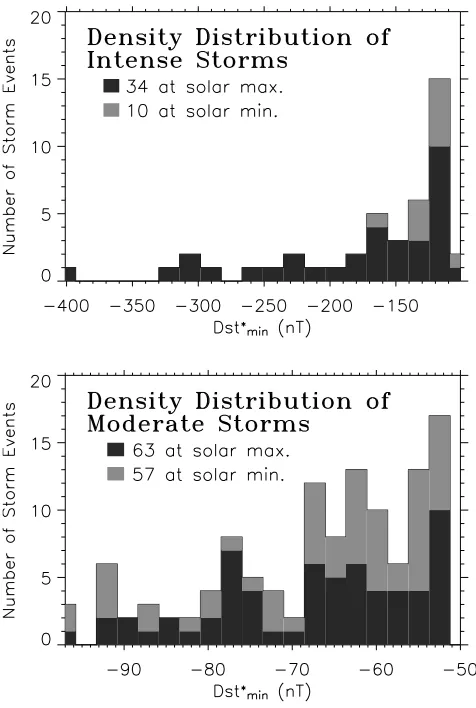
[12] Figure 2 shows the density distribution of the two

levels of storm intensity at the two solar extrema. In each

Figure 1. Histogram of the number of moderate and

intense storm events at solar minimum (July 1994 – June 1997) and solar maximum (July 1999 – June 2002). The total of storms is parenthesized in the figure title. The numbers in other parentheses indicate the subtotal of storms in each category.

Figure 2. Density distribution of intense storms (upper) and moderate storms (lower) at solar maximum and at solar minimum. Dst*min is minimum Dst* value of each storm.

Figure 3

storm category, the peak of the density distribution occurs near the upper limit of theDst* range for event identifica-tion, that is, 100 nT in intense storms and 50 nT in moderate storms. The minimumDst* (Dst*min) values of the

two most intense storms at solar minimum reached only

131.6 nT and154.2 nT. The intensity of all other intense storms at solar minimum is >125 nT. As for the 34 intense storms at solar maximum, six of them are super-storms (Dst*min 250 nT).

3. Data Analysis

[13] Superposed epoch analyses of the four

energy-channel fluxes and four derived bulk parameters of hot ions at geosynchronous orbit are performed for each of the four storm categories: intense storms at solar maximum, intense storms at solar minimum, moderate storms at solar maximum, and moderate storms at solar minimum. In the companion work, Zhang et al. [2006] used the same statistical technique to study the average behaviors of solar wind plasma and IMF parameters, NOAA/POES Hemispheric Power, Kp, and Dst* in the four storm categories with storms in Solar Cycle 21 and 22 also included.

[14] Dst*min is taken as the zero epoch of the superposed

epoch analyses and the time domain is ±1.5 days. In other words, the epoch time period is from 1 1/2 days before Dst*minto 1 1/2 days afterward. For each storm category, the

eight MPA parameters observed by all the six LANL satellites, as a function of local time (LT) and universal time (UT), are grouped into 1-hour square bins, respectively. The MPA values in each LT-UT bin are then averaged.

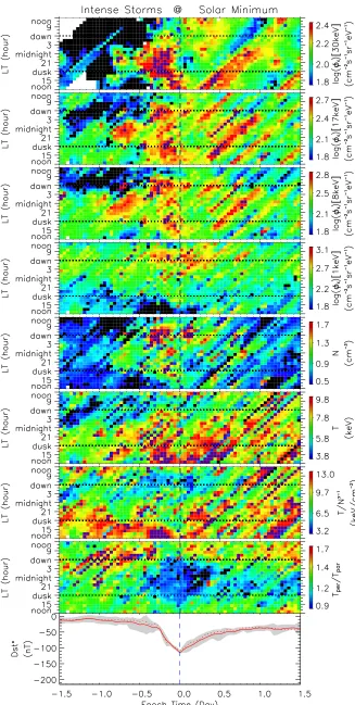
[15] From top to bottom, Figure 3 shows the superposed

epoch averages of the base-10 logarithms, denoted by ‘‘log’’ in the text below, of the fluxesf(with energies30,17,

8, and1 keV), and linear scales for the number density N, temperature T, entropyT/Ng1, and temperature anisot-ropyTper/Tparof hot ions before and during intense storms at solar maximum. The vertical dotted line denotes the zero epoch,Dst*min. The means, medians, first quartiles, and third

quartiles of Dst* are also shown in the last panel. The averaged MPA data are color coded in the local time versus universal time plots (LT-UT maps) because LT-UT maps are a good method of displaying the large amounts of MPA data. Statistics like standard deviations and quartiles from the superposed epoch analyses of the MPA parameters are not shown but can be provided upon request from the authors. On the LT-UT maps, bins with missing data are colored white, and black (purple) bins indicate that the values are lower (higher) than the minimum (maximum) of the corresponding color bar. Between the two horizontal

dotted lines on the LT-UT maps of the MPA data is the nightside, that is, 1800 LT to 0600 LT which is centered around midnight.

[16] Similarly, Figures 4, 5, and 6 show the results of the

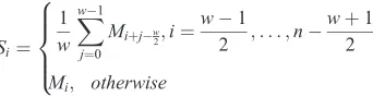
superposed epoch analyses in the other three storm catego-ries, respectively. For convenience in making comparisons, the range of the color bar in every MPA LT-UT map and the Y axis ranges in the Dst* panels are the same among Figures 3 – 6. In Figure 4, because of large geosynchro-nous-orbit observation gaps due to only ten intense storms at solar minimum, white bins on the LT-UT maps of the MPA data are filled with linearly smoothed values which are computed by the following algorithm:

Si¼

1

w

X w1

j¼0

Miþjw 2;i¼

w1

2 ;. . .;n

wþ1 2

Mi; otherwise 8 > > < > > :

whereMiis the averaged MPA parameter value in theith LT or UT bin on an LT-UT map,nis the total of LT or UT bins on the LT-UT map,wis the width of the smoothed window, and Si is the smoothed result of Mi. Thus the smoothing formula is applied for both LT and UT bins. If a neighbor bin is found to be outside the LT-UT map, values in the nearest edge bin are used to compute the smoothed results. In our calculation, w is set to 5; however, there are still white areas (no data available) in the LT-UT maps of Figure 4 when the gap was larger thanw.

[17] Table 1 quantitatively gives the average peak values

of hot-ion parameters at geosynchronous orbit andDst*min

in the four storm categories. After each mean is the corresponding standard deviation. Detailed comparisons of those peak values will be made in the following text.

[18] To test the statistical significance of the means in

Figures 3 – 6, we calculate the Student’s t-statistic and its significance [Reiff, 1990] for each MPA parameter in every 1-hour LT-UT bin among the four storm categories.Zhang et al.[2006] also made the same Student’st-test calculations on all IMF and solar wind plasma parameters and geomag-netic indices likeDst*,Kp, and NOAA/POES Hemispheric Power. The Student’st-statistict of population xand y is defined as

t¼ _{ffiffiffiffiffiffiffiffiffiffiffiffiffiffiffiffiffiffiffiffiffiffiffiffiffiffiffiffiffiffiffiffiffiffiffiffi}xy

P

M1

i¼0 xix

ð Þ2_þP N1

i¼0 yiy

ð Þ2

MþN2

s 1 Mþ 1 N ;

where x = (x0, x1, x2, . . ., xM1) with mean x and y =

(y0, y1, y2, . . ., yN1) with mean y. The significance of

Figure 4. Same format as Figure 3, but for intense storms at solar minimum.

Figure 6. Same format as Figure 3, but for moderate storms at solar minimum.

the Student’s t-statistic, p, is determined by the incom-plete ibeta function

Ixða;bÞ ¼ Rx

0u

a1_ð1uÞb1_du

R1

0ua1ð1uÞ

b1_du;

which is the probability that the absolute value oftcould be at least as large as the computed statistic given a random data set. The means of x and y are considered to be significantly different ifp< 0.05 [Miller, 1986;Press et al., 1992]. However, the Student’s t-test assumes thatx andy have the same true variance. If xandyhave very different variances, the difference of x and y may be difficult to interpret [Press et al., 1992].

[19] Results from the Student’s t-test show that visual

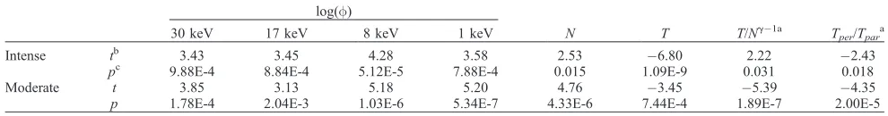
inspection is good enough to determine whether features on the LT-UT maps are statistically different (p< 0.05). One possible reason is that means in most of those 1-hour LT-UT bins are calculated from as many as 1500 data points because of the richness of the MPA database. Note that the MPA data resolution is 86 s. Similar to Table 1 of Zhang et al. [2006], Table 2 lists some results of the Student’s t-test for the peaks of each hot-ion parameter between half a day before and after Dst*min during intense

storms and moderate storms between the two solar extrema, respectively. If peaks do not appear in the same bin on an LT-UT map, which is true in most cases, the Student’st-test is done for the peak value at solar maximum and the nonpeak value at the same local time and universal time at solar minimum. If peaks are found to be different from

each other by eye, then the t-statistic significance, p, is always far smaller than 0.05, as shown in Table 2.

4. Results: Similarities and Differences 4.1. Similarities

[20] Figures 3 – 6 demonstrate the typical features of four

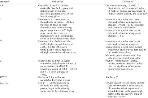
different energy channels of fluxes, density, temperature, temperature anisotropy, and entropy of geosynchronous-orbit hot ions and theDst* statistics (means, medians, first and third quartiles from the superposed epoch analysis) prior to and during intense storms and moderate storms at solar maximum and at solar minimum, respectively. Some features of the hot-ion parameters are in agreement with previous studies [e.g., McIlwain, 1972; Borovsky et al., 1997a, 1997b; Borovsky et al., 1998b; Kozyra et al., 1998b; Thomsen et al., 1998a, 1998b, 2003; Wing and Newell, 1998; Korth et al., 1999; Korth and Thomsen, 2001; Friedel et al., 2001; Fok et al., 2003;Ebihara and Fok, 2004;Ebihara et al., 2005;Denton et al., 2005, 2006], while others are presented here for the first time. TheDst* panel is shown only for reference.Zhang et al.[2006] have reported the similarities and differences ofDst* in the four storm categories. Table 3 outlines the similarities, discussed in detail as follows, on the LT-UT maps of the four storm types for each hot-ion parameter.

[21] As shown in the LT-UT maps of Figures 3 – 6, during

the epoch time period of 3 days, all the geosynchronous-orbit hot-ion parameters vary with both local time (LT) and universal time (UT). In other words, each of them is a function of LT and UT. Moreover, during the average main phase and the early average recovery phase (about half a Table 1. Average Peak Values of Hot-Ion Properties at Geosynchronous Orbit andDstmin* in Each Storm Category

Parameters Intense @ Max. Intense @ Min. Moderate @ Max. Moderate @ Min. log(f)[30 keV] cm2s1sr1eV1 2.55 ± 0.20a 2.61 ± 0.05 2.34 ± 0.22 2.44 ± 0.11 log(f)[17 keV] cm2_s1_sr1_eV1 _{2.73 ± 0.20 3.12 ± 0.05 2.61 ± 0.26 2.63 ± 0.27}

log(f)[8 keV] cm2s1sr1eV1 2.81 ± 0.19 3.03 ± 0.12 2.66 ± 0.21 2.66 ± 0.09 log(f)[1 keV] cm2_s1_sr1_eV1 _{3.16 ± 0.17 3.52 ± 0.43 2.90 ± 0.29 2.80 ± 0.48}

Ncm3 2.33 ± 0.64 2.92 ± 0.19 1.47 ± 0.55 1.42 ± 0.73

TkeV 9.65 ± 2.50 13.59 ± 0.62 9.77 ± 2.15 10.38 ± 1.61

T/Ng1keV/cm2 13.27 ± 2.59 25.51 ± 2.45 14.22 ± 3.72 15.93 ± 4.33 T/Ng1b_keV/cm2 _{1.88 ± 0.79 0.88 ± 0.07 3.87 ± 1.95 4.17 ± 1.07}

Tper/Tparb 0.87 ± 0.13 0.64 ± 0.05 0.91 ± 0.19 0.73 ± 0.22

Dst*minnT 169.08 ± 74.35 115.53 ± 16.81 66.51 ± 12.26 64.43 ± 12.39 a

Here ±1 standard deviations are shown behind the plus-minus signs.

b_{Shown are minima ofT/N}g1_orT

per/Tpar, not peak values.

Table 2. Student’st-Test for Peaks in 0.5-day Before and AfterDst*minDuring Intense Storms and Moderate Storms Between at Solar

Maximum and at Solar Minimum

log(f)

N T T/Ng1a Tper/Tpar a

30 keV 17 keV 8 keV 1 keV

Intense tb 3.43 3.45 4.28 3.58 2.53 6.80 2.22 2.43

pc _{9.88E-4 8.84E-4 5.12E-5 7.88E-4 0.015 1.09E-9 0.031 0.018}

Moderate t 3.85 3.13 5.18 5.20 4.76 3.45 5.39 4.35

p 1.78E-4 2.04E-3 1.03E-6 5.34E-7 4.33E-6 7.44E-4 1.89E-7 2.00E-5

a

As forT/Ng1andTper/Tpar, Student’st-test is for minima, not for peak values. b_{Heretstands for the Student’st-statistic.}

c

day before and after Dst*min) in each of the four storm

categories, every hot-ion parameter is disturbed around Dst*min. They display obvious regions of increase or

de-crease and show distinct peaks or minima. Furthermore, the locations of these increase or decrease patterns do not change much with levels of geomagnetic activity either at solar maximum or at solar minimum. These storm-time disturbances of the hot-ion parameters are in response to the enhancement of upstream IMF components, solar wind plasma parameters, and motional electric field in the four storm categories as presented byZhang et al.[2006]: (1) the southward IMFBzand associated electric field exceed a key threshold value for a long duration; (2) the IMF magnitude is enhanced and the three IMF components are all disturbed; and (3) the solar wind density, bulk flow speed, dynamic pressure, and temperature begin to increase several hours beforeDst*min. Corresponding geomagnetic activity in each

storm category is also consistently exhibited in the average behaviors of NOAA/POES Hemispheric Power, Kp, and Dst* during storms [Zhang et al., 2006].

[22] As one can see on the first panels of Figures 3 – 6, the

ion fluxes for the higher-energy channel (30 keV) are enhanced during almost the whole nightside in the main phase. However, when the channel energy drops from

17 keV, 8 keV, to1 keV, the enhancement begins to shift close to the dawnside and extend into the early recovery phase. The regions with low fluxes (blue or black bins) also change from the morning sector at higher energies to the afternoon sector at1 keV. Especially, at an energy of 1 keV, ion flux rates near dawn are unusually higher

than those near dusk during half a day before and after Dst*min; however, a few hours afterDst*min, the ion fluxes at 30 keV are higher on the duskside than on the dawnside. In addition, one can see higher peak flux rates in the lower-energy channels, which is also shown in Table 1. The only exception is found during intense storms at solar minimum; the averaged log flux at 17 keV, which is 3.12 (flux unit: cm2s1sr1eV1) as in Table 1, is larger than that at 8 keV, 3.03, but they are statistically the same if the standard deviations, 0.05 and 0.12, respectively, are con-sidered. Another interesting aspect of the hot-ion fluxes is that in the earlier recovery phase the flux rates in every channel are low in the premidnight sector. This feature is more obvious during intense storms than during moderate storms; it is not apparent during moderate storms at solar maximum.

[23] As shown on the fifth LT-UT map of Figures 3 – 6,

hot-ion density is enhanced 24 hours before and afterDst*min

in each type of storm. The density enhancement also has LT dependence; it always falls off close to noon. Furthermore, in the early morning sector and the postmidnight sector (midnight – 0900 LT) and for a UT interval, 12 hours before and afterDst*min, the hot ions are extraordinarily dense, with

average peak values as high as 1.47 cm3 for moderate storms and 2.92 cm3 for intense storms. This feature makes the hot-ion density have a clear asymmetric LT distribution around Dst*min during storms, which is also

noted by several previous studies [e.g.,Korth et al., 1999; Liemohn et al., 2001;Fok et al., 2003;Ebihara et al., 2005; Denton et al., 2005, 2006]. However, during low geomag-Table 3. Outline of the Results in Section 4

Parameters Similarities Differences

All Vary with LT and UT; display obviously disturbed regions with distinct peaks or minima; recover to prestorm levels in the late recovery phase

Disturbance intensity, LT and UT distributions, and location and value of peaks or minima are dependent on levels of storm intensity and solar activity.

f Enhanced in the main phase on

the nightside in channel30 keV but close to dawn in other channels; lower in the morning sector except for1 keV; higher peak rates in lower-energy channels; low in the premidnight sector in the earlier recovery phase

Intense storms at solar min.: most extended enhancement regions in channel30 and17 keV; highest peak values in each channel Intense storms at solar max.: most

extended enhancement regions in channel1 keV

N Enhanced 24 hrs before and after Dst*min; higher around dawn and

Dst*min, but fall off close to

noon; at quiet times, peak near midnight and minimized near noon

Intense storms at solar max.: most extended enhancement regions Intense storms at solar min.: highest

peak value; another peak near dusk in the middle main phase

Moderate storms at solar min.: less enhanced and lowest peak value T Higher in the 12-hour LT sector

centered at dusk than the 8-hour LT sector centered at 0700 LT; lowest in a region at 0700 – 1000 LT and 8 UT hours centered at Dst*min

Highest (second highest) during intense (moderate) storms at solar min.; no significant enhancement during solar max. storms

T/Ng1 Similar toT, but with more remarkable low-value regions

Similar toT

Tper/Tpar Low (=1) on the nightside in

the main and early recovery phases; larger in the morning sector than in the afternoon sector

Lowest (second lowest) during intense (moderate) storms at solar min.; no obvious dawn-dusk asymmetry; a second decrease in the premidnight sector in the late reovery phase of solar min. storms

netic activity, it was found that hot-ion density peaks near local midnight, drops toward both dawn and dusk and is minimized near noon [DeForest and McIlwain, 1971; Garrett et al., 1981; Thomsen et al., 1996b; Maurice et al., 1998]. This quiet-time LT variation is consistent with those in the first and last 12 epoch hours on the density LT-UT maps in Figures 3 – 6.

[24] From 0300 to 1100 LT (through dawn; total 8 local

hours), hot-ion temperature is generally lower than that at other local times during almost the entire 3-day epoch time. Interestingly, each temperature LT-UT map of Figures 3 – 6 shows a very cool region at 0700 – 1000 LT and ±4-hour epoch time centered atDst*min. The temperature can be as low

as 2.60, 2.31, 4.12, and 3.62 keV in this region, compared to peak values at 9.65, 13.59, 9.77, and 10.35 keV in Table 1 for intense storms at solar maximum, intense storms at solar minimum, moderate storms at solar maximum, and moderate storms at solar minimum, respectively.

[25] Hot-ion entropy has similar LT-UT maps to those of

temperature. That is, the temperature and the entropy are almost consistently higher in the 12-hour LT sector centered at dusk than the 8-hour LT sector centered at 0700 LT. Nevertheless, during intense storms either at solar maxi-mum or at solar minimaxi-mum, the regions of low entropy are even more remarkable than the regions of low temperature because entropy is calculated fromT/Ng1and, as discussed above, hot-ion density has distinct enhancements near dawnside around Dst*min. As shown in Table 1, the lowest

entropy during intense storms is 1.88 keV/cm2 at solar maximum and 0.88 keV/cm2at solar minimum, but it is 3.87 keV/cm2and 4.17 keV/cm2during moderate storms at solar maximum and at solar minimum, respectively.

[26] Temperature anisotropy also has two prominent

features. One feature is that Tper/Tpar is significantly re-duced during disturbed times on the nightside with a minimum near midnight. That is, Tper/Tpar is low (=1) on the entire nightside in the main phase and the early recovery phase. In other words, at geosynchronous orbit, isotropic hot ions extend across the nightside during storms, but they become anisotropic (Tper/Tpar> 1) close to noon. The other feature is thatTper/Tpar in the morning sector is usually larger than that in the afternoon sector in each storm category.

[27] As the storm driver, a southward IMF, becomes

weaker and has a northward turning in the end [Zhang et al., 2006], the large-scale magnetospheric convection is reduced and the mass and energy transport from the solar wind to the magnetosphere decreases. Finally, in the late recovery phase (the last 24 hours of the 3-day epoch time), almost all enhanced or decreased hot-ion parameters recover to their prestorm levels when various losses, such as charge exchange, atmospheric losses, Coulomb collisions, etc. [e.g., Kistler et al., 1989; Fok et al., 1991; Jordanova et al., 1996;Kozyra et al., 1998a], remove energetic particles from the ring current.

4.2. Differences

[28] In addition to having many features in common, the

LT-UT maps in Figures 3 – 6 also illustrate the differences of the average variations of the four energy-channel flux rates, density, temperature, temperature anisotropy, and entropy of geosynchronous-orbit hot ions among the four storm

cate-gories. Consistent with the average solar wind conditions [Zhang et al., 2006], the disturbance intensity and LT and UT distributions of the hot-ion parameters have dependence on the levels of geomagnetic activity and solar activity. Table 3 also outlines the differences, discussed in detail as follows, on the LT-UT maps of the four storm types for each hot-ion parameter.

[29] The exact location (both LT and UT) and value of the

peaks or minima change with levels of storm intensity either at solar maximum or at solar minimum. For example, during intense storms at solar maximum, the log fluxes at the energy of30 keV peak at 2.55 4 hours earlier thanDst*min

in the postmidnight sector (at LT = 0400, precisely). However, the log fluxes in the same channel during intense storms at solar minimum have a peak value of 2.61 between dusk and local midnight. In the 1-hour LT-UT bin where intense storms at solar maximum have the flux maximum at

30 keV, the log fluxes at the same energy in the other three storm classes are relatively low: 2.31 during intense storms at solar minimum, 2.10 during moderate storms at solar maximum, and 1.88 during moderate storms at solar mini-mum. The Student’st-tests indicate that 2.55 is significantly different from these values:t= 3.43 andp= 9.88E-4 (also listed in Table 2),t= 5.95 andp= 1.16E-8, andt= 2.35 and p = 2.07E-2, respectively, at a confidence level of nearly 100%.

[30] On the flux LT-UT maps of Figures 3 – 6, one can see

that intense storms at solar minimum have the most extended increase regions of fluxes at 30 and 17 keV in the main phase and the early recovery phase; however, the extent of increase regions of fluxes at 8 keV during intense storms at solar maximum is comparable to that during intense storms at solar minimum. As far as the last channel is concerned, it is obvious that the most extended increase regions at1 keV are on the LT-UT map of intense storms at solar maximum. As shown in Table 1, even though intense storms at solar minimum are not on average the most intense [Zhang et al., 2006], i.e., the averaged Dst*min is larger than that of intense storms at solar

maxi-mum by more than 50 nT, the averaged peak value of log flux at30 keV, 2.61, is the highest in the four categories. This is true in the other three channels of fluxes; intense storms at solar minimum always have the highest average flux rates at 17 keV,8 keV, and1 keV. The second largest fluxes in all the four channels are always around Dst*minof intense storms at solar maximum. As for moderate

storms, like their similar averaged Dst*min [Zhang et al.,

2006], the peak flux rates in each channel are not much different from each other.

[31] Although the dawnside enhancement regions of the

absolute value of the averageDst*min among the four types

of storm as indicated in Table 1. In Figure 3, one can see another special feature of intense storms at solar minimum: density, as well as fluxes at30,17, and8 keV, exhibits another peak near dusk in the middle of the main phase.

[32] On the nightside and in the afternoon sector,

geo-synchronous-orbit-altitude ions in the main phase and recovery phase of intense storms at solar minimum are generally the hottest in those enhanced temperature regions, more red and purple bins, among the four storm categories. The second hottest hot-ion regions are also, surprisingly, found during the other type of solar minimum storm, i.e., moderate storms at solar minimum. As a matter of fact, one can not see significant temperature enhancements during solar maximum storms, especially during intense storms at solar maximum. Peak temperature values given in Table 1 further confirm this difference: 9.65 keV during intense storms at solar maximum, 13.59 keV during intense storms at solar minimum, 9.77 keV during moderate storms at solar maximum, and 10.38 keV during moderate storms at solar minimum.

[33] A very similar feature can also be found in entropy

on the LT-UT maps of Figures 3 – 6. Moreover, as shown in Table 1, the average entropy during intense storms at solar minimum, 25.51 keV/cm2, is extraordinarily high; it is larger than those in other storm classes by more than 9 keV/cm2. The second largest entropy (15.93 keV/cm2) and the lowest value of the entropy peaks (13.27 keV/cm2) are also found during moderate storms at solar minimum and during intense storms at solar maximum, respectively.

[34] As listed in Table 1, intense storms (moderate

storms) at solar minimum again have the lowest (the second lowest) average anisotropy, 0.64 (0.73), among the four storm categories. As shown in Figures 3 – 6, the most remarkable feature of temperature anisotropy is that its decrease regions spread across the entire nightside, and it then does not show distinct dawn-dusk asymmetry like other parameters. In the late recovery phase during both intense storms and moderate storms at solar minimum, temperature anisotropy decreases a second time in the premidnight sector. More data are necessary to verify whether this is a typical feature during solar minimum storms.

5. Discussion

[35] In this paper, using the superposed epoch technique

as in the companion study of [Zhang et al., 2006], we have examined and compared the average behaviors of the hot-ion properties (fluxes, moments, and their derivatives) at geosynchronous orbit during intense storms and moderate storms at solar maximum and at solar minimum of Solar Cycle 23. After the large amounts of the MPA data are averaged and then color coded on the LT-UT maps, the timing and asymmetry/symmetry of intensifications in the quantity of each hot-ion parameter are readily apparent. The similarities and differences of those average patterns among the four storm categories have important implica-tions for the purpose of understanding the storm-time ring current sources. Moreover, the statistical results from the MPA data analysis can be applied to obtain better simula-tion results because the geosynchronous-orbit plasmas are often used as an outer boundary for modeling the inner magnetosphere, especially the storm-time ring current.

[36] In order to include as many storm events as possible

in our study, we define solar maximum and solar minimum of Solar Cycle 23 exactly the same way as in the companion work by Zhang et al. [2006]. That is, solar minimum (maximum) is the time period of 3 years approximately centered on the trough (crest) of the monthly smoothed sunspot numbers in Solar Cycle 23. Therefore the usual solar minimum (maximum) [e.g.,Vennerstroem, 2001] and a short period of the late (early) declining phase and the early (late) rising phase of the solar cycle have been chosen as the duration of solar minimum (maximum) in this paper. However, even with the loose definition of solar minimum, the superposed LT-UT maps of intense storms at solar minimum are produced with only 10 events. In order to test the statistical significance, we conducted the Student’s t-test on the means in each LT-UT bin among the four storm categories. Since there are fewer geosynchronous LANL satellites in earlier years (e.g., at solar minimum), the Student’st-test is a good alternative to ensure that compar-isons among the results are significant, even with a rela-tively small number of storms.

5.1. Access to Geosynchronous Orbit and Fluxes

[37] During storms, responding to the strong southward

IMF and other accompanying disturbances in upstream solar wind plasma and IMF as presented by Zhang et al. [2006], the plasma sheet can access geosynchronous orbit under the enhanced large-scale convection electric field [Zhang et al., 2001;Korth et al., 1999;Korth and Thomsen, 2001]. As a result, more energetic and denser particles in the plasma sheet become the typical plasma populations in part of the geosynchronous orbit in the main phase and in the early recovery phase of storms, which are detected by the MPA instruments. In other words, those energized ions and electrons from the plasma sheet can be transported across geosynchronous orbit to closer to the Earth (typically, L = 3 – 6). This deep plasma penetration is consistent with the storm-time enhancement of NOAA/POES Hemispheric Power and the intensity of the ring current that is gauged by the averageDst* and Kp as presented by Zhang et al. [2006]. The typical properties of low-energy ions and electrons at geosynchronous orbit were investigated in several previous studies [e.g., Korth et al., 1999; Denton et al., 2005, 2006]. The LT and UT dependence of the hot-ion properties at geosynchronous orbit is the focus of this present paper.

[38] Unlike cold ions and electrons, hot ions have very

complex drift paths in the inner magnetosphere, which are dependent on levels of geomagnetic activity and their magnetic moments (the first adiabatic invariant)

m¼

1 2mv2?

B ;

where mv?2/2 is the kinetic energy perpendicular to the magnetic field B, and B is the magnitude of B. Using a simple Alfve´n layer model, Korth et al. [1999] computed the position of the separatrix between open and closed ion drift paths as a function of energy, local time, and level of geomagnetic activity. At quiet times (Dst* 50 nT), geosynchronous orbit is located in the region of closed drift paths for ions at energies greater than30 keV. In this case,

the stagnation point is on the dawnside. At lower ion energies, the corresponding separatrix first moves closer to the Earth, then evolves into two sets with one being a closed banana orbit, and lastly reverses its configuration with the stagnation point flipping to the duskside [Korth et al., 1999, Figure 1]. In other words, under low geomagnetic activity, very hot ions in the plasma sheet do not have access to geosynchronous orbit; for intermediately hot ions, the plasma sheet can have access to geosynchronous orbit in the premidnight sector and the afternoon sector; for lower-energy ions, the plasma sheet begins to access geosynchro-nous orbit from the other side, i.e., from the postmidnight sector and the morning sector. Therefore as shown on the flux LT-UT maps, low flux rates at30,17, and8 keV are found in the morning sector but those at1 keV are in the afternoon sector. During storms, for hot ions in each channel, the separatrix goes even closer to the Earth than that of same-energy ions at quiet times and the banana orbit appears in the drift paths of lower-energy ions. Thus

30 keV ions in the plasma sheet can be injected inside of geosynchronous orbit in the main phase to make the flux rates at 30 keV enhanced across nearly the entire nightside. Similarly, the theoretical locations of the separatrix in other channels can be used to explain the dawnside shift of the flux enhancements at the energy from

17 keV,8 keV, to1 keV.Ebihara and Fok[2004] also studied the postmidnight storm-time enhancement of tens-of-keV proton fluxes from the IMAGE satellite, but they did not consider the effects of the energy dependence of proton drift paths on the flux LT distributions.

[39] Note that the Alfve´n layer model is highly simplified.

The realistic ion injections into the inner magnetosphere passing geosynchronous orbit are much more complicated. Several other factors can affect the LT and UT distributions of hot-ion flux rates in geosynchronous orbit. First of all, loss processes such as charge exchange, atmospheric losses, wave-particle interactions, and Coulomb collisions [e.g., Kistler et al., 1989; Fok et al., 1991; Jordanova et al., 1996; Kozyra et al., 1998a] play an important role in causing the dawn-dusk asymmetry of the flux LT distribu-tions because plasma sheet ions take drift paths with different lengths to arrive at dawn and at dusk. Those ions with longer and more circuitous routes suffer more losses and hence have lower flux rates [Korth et al., 1999]. This may be a reason for why in the earlier recovery phase of each type of storm the flux rates in every channel are almost always low in the premidnight sector. The hot-ions presum-ably have experienced losses before they are injected from the magnetotail and reach the premidnight sector. Second, particles closer to the stagnation point have slower flow speeds; particles are expected to stagnate at the stagnation point. Hot-ion fluxes near the stagnation point can be enhanced during storms. Third, at most times, there is a partial ring current during the storm main phase. Additional charging, positively at dusk and negatively at dawn, occurs on the nightside. The resulting dusk-dawn polarization electric field shields the near-Earth region from the dawn-dusk convection electric field and opposes the convection in the inner magnetosphere. Overshielding (undershielding) occurs when the driving convection electric field is suddenly reduced (increased), due to the sudden changes in southward IMF magnitude or sign [e.g., Spiro et al., 1988;Fejer and

Scherliess, 1997; Goldstein et al., 2003]. The flux LT asymmetry can result from these shielding phenomena. However, further investigations are needed to examine the detailed physical processes and to see which of these mechanisms dominates. Last, the plasma transport via the low-latitude boundary layer (LLBL) into the magnetosphere may also have effects on the dawn-dusk asymmetry in the hot-ion fluxes. The solar wind plasma, first trapped in the magnetosheath, can enter the plasma sheet through both the high-latitude lobes and the LLBL. It has been found that the portion of plasma entering via the LLBL is both dense and cold [e.g.,Eastman et al., 1976;Fujimoto et al., 1996, 1998a, 1998b]. These cold, dense ions, which have the plasma characteristics of the magnetosheath, are found to be present close to the dawnside in the morning sector aroundDst*minon the density and temperature LT-UT maps

in each of the four storm categories.

5.2. Bulk Properties

[40] Hot-ion density has been calculated according to

measured fluxes in 14 channels with an energy range from

0.1 to 45 keV. Because the ion drift trajectories are energy dependent, as found in our statistical results, the locations of the flux enhancement regions at different levels of energies are different from each other. When energies become lower, those enhancement regions shift from the entire nightside to dawnside and show a distinct dawn-dusk asymmetry. Moreover, higher flux peak values are found in the lower-energy ions. As a result, the calculated density is contributed more from the portions of ions with lower energies. During storms, the dawn-dusk asymmetry in density is determined by (and thus similar to) that of the lower-energy ion fluxes. Considering the complexity, espe-cially the energy dependence, of ion drifts in the inner magnetosphere, it would have limitations in investigating only the ion bulk properties and ignoring the energy dependence of the ion drift paths to understand the devel-opment of the ring current.

[41] The locations of the regions with high density, low

temperature, and low entropy indicate that the delivery of fresh (cold and dense) ions into the inner magnetosphere has an obvious LT asymmetry. As discussed above, 0300 – 1100 LT on the dawnside is the region where the cold and dense ions are transported from the solar wind through the magnetosheath and LLBL into geosynchronous orbit. Because collisions are frequent on the nightside and there is no preferred direction, hot ions are isotropic on the entire nightside during storms and do not show a clear dawn-dusk asymmetry. In other words, on the nightside, the thermal speed of hot ions along the magnetic field direction is not different from that perpendicular to the magnetic field direction. However, on the dayside, especially in the morn-ing sector, the perpendicular speed of hot ions can be higher than the parallel one.

[42] The LT asymmetries in fluxes, density, temperature,

the effects of the LT asymmetries on the ring current depend on different solar wind conditions.

5.3. Solar Cycle Dependence

[43] Borovsky et al.[1998a] found that the properties of

the plasma sheet are highly correlated with the properties of the solar wind. Therefore hot-ion properties at geosynchro-nous orbit during storms show dependence on the solar cycle. The plasma sheet density and the solar wind density correlate to each other with a correlation coefficient as high as 0.67 [Borovsky et al., 1998a]. In addition, the statistical companion study by Zhang et al. [2006] shows that solar wind density in the main phase of intense storms at solar minimum is on average the highest in the four storm categories. This is consistent with the fact that the highest plasma sheet density is found in intense storms at solar minimum, even though the broadest density enhancement region is shown on the LT-UT map of intense storms at solar maximum.

[44] In the magnetosphere, the primary energy transfer

process is mechanical energy from the solar wind flows being converted into magnetic energy and stored in the magnetotail. The magnetic energy is then converted into mostly thermal mechanical energy in the plasma sheet, auroral particles, ring current, and Joule heating in the ionosphere [Gonzalez et al., 1994]. Borovsky et al. [1998a] found that the temperature of the nightside plasma sheet is correlated with the speed of the solar wind with a linear correlation coefficient as high as 0.56. At solar maximum, coronal mass ejections (CMEs), of which one-third to one-half are magnetic clouds (MCs), play an overriding role in driving geomagnetic storms [e.g., Tsurutani and Gonzalez, 1997;Gonzalez et al., 1999;Zhang et al., 2004]. However, at solar minimum, the dominating geoeffective solar wind structures are corotating interaction regions (CIRs) [e.g., Tsurutani and Gonzalez, 1997; Gonzalez et al., 1999], associated with very high-speed streams. High-speed solar wind flows, originating from open solar magnetic field lines at solar minimum, may be one of the reasons for the higher ion temperature in the afternoon sector and on the nightside at geosynchronous orbit during solar minimum storms than during solar max-imum storms. However, extremely fast solar winds are mostly observed in the ejecta (CMEs or MCs); moreover, it is found in the companion study by Zhang et al.[2006] that solar wind flows in the 3-day epoch time of intense storms at solar minimum are on average the slowest among the four storm categories. One possibility for this difference is thatZhang et al.[2006] did not choose the zero epoch at CIR interfaces, and thus average speeds at several time points were calculated from both high-speed flows and low-speed flows. Other than this one, we have no other reason-able explanations for the inconsistency in the two recent studies. Further investigation is needed to figure out why hot-ion temperature and entropy are on average not clearly enhanced during solar maximum storms.

6. Summary

[45] We summarize our statistical survey of the hot-ion

properties at geosynchronous orbit during the 164 storms in the four categories as follows:

[46] 1. Fluxes (at30,17,8, and 1 keV), density,

temperature, entropy, and temperature anisotropy vary with both local time (LT) and universal time (UT). In the main phase and the early recovery phase during storms, respond-ing to the upstream geoeffective IMF and solar wind parameters, all hot-ion parameters are highly disturbed around Dst*min; they display obvious increase or decrease

regions and show distinct peaks or minima. In addition, the locations of these increase or decrease patterns do not change much with levels of geomagnetic activity and solar activity.

[47] 2. Fluxes at30 keV are enhanced during almost the

entire nightside in the main phase; as the energy is reduced to17,8, and to1 keV, the enhancement begins to shift close to dawn and also extend into the early recovery phase. Furthermore, the lower the channel energy, the higher the flux peak values. The regions with low fluxes also change from the morning sector at higher energies to the afternoon sector at1 keV.

[48] 3. Similar to their uncommon superposed solar wind

driver [Zhang et al., 2006], intense storms at solar minimum always have the highest (lowest) average peak value (min-imum) in each hot-ion parameter among the four storm categories, even though their average ring current is not the most intensified; in this storm category, density and fluxes at30,17, and8 keV exhibit another peak near dusk in the middle of the main phase.

[49] 4. During each type of storm, density has a clear

asymmetric LT distribution around Dst*min; it peaks in a

region of 0900 LT – midnight and 12 UT hours before and after Dst*min and falls off close to noon. During moderate

storms at solar minimum, density has the lowest peak value and is least enhanced in the whole 3-day epoch time among the four storm categories, which is consistent with the fact that the averageDst*minin this storm category is the lowest.

[50] 5. From 0300 LT through dawn to 1100 LT,

temper-ature and entropy are generally lower than those at other local times during nearly the entire 3-day epoch time. Very low temperature and entropy are found in a region of 0700 – 1000 LT and ±4-hour epoch time centered at Dst*min.

Because high-speed solar winds dominate at solar mini-mum, in their enhanced regions (nightside and afternoon sector), both temperature and entropy during solar minimum storms are usually higher than those during solar maximum storms; there is actually no clear temperature and entropy enhancement during solar maximum storms.

[51] 6. During storms, hot ions are isotropic on the

nightside but anisotropic (Tper/Tpar> 1) close to noon. In the late recovery phase during solar minimum storms, temperature anisotropy decreases a second time in the premidnight sector.

[52] 7. In the late recovery phase in every storm category,

along with IMFBsbecoming weaker and turning northward, almost all enhanced or decreased hot-ion parameters recover to prestorm levels.

[53] Acknowledgments. We would like to thank WDC-C2, Kyoto for providing theDstindex. Solar wind density and bulk flow speed used to calculateDst* were obtained from the Wind and ACE spacecrafts through the NSSDC in NASA Goddard Space Flight Center. We also gratefully acknowledge other MPA team members for helping prepare the MPA data. This work was supported by NSF under grant number ATM-0402163 and NASA under grant numbers NNG05GJ89G and NNG05GM48G. The work

of M. F. Thomsen, M. H. Denton, and J. E. Borovsky at LANL was carried out under the auspices of the U. S. Department of Energy, with partial support from the NASA LWS program, under subcontract to the University of Michigan.

[54] Amitava Bhattacharjee thanks Larry Lyons and another reviewer for their assistance in evaluating this paper.

References

Akasofu, S.-I. (1981), Energy coupling between the solar wind and the magnetosphere,Space Sci. Rev.,28, 121 – 190.

Balsiger, H., P. Eberhardt, J. Geiss, and D. T. Young (1980), Magnetic storm injection of 0.9 – 16 keV/e solar and terrestrial ions into the high-altitude magnetosphere,J. Geophys. Res.,85, 1645 – 1662.

Bame, S. J., D. J. McComas, M. F. Thomsen, B. L. Barraclough, R. C. Elphic, and J. P. Glore (1993), Magnetospheric plasma analyzer for spacecraft with constrained resources,Rev. Sci. Instrum.,64, 1026 – 1033. Baumjohann, W. (1993), The near-Earth plasma sheet: An AMPTE/IRM

perspective,Space Sci. Rev.,64, 141 – 163.

Baumjohann, W., G. Paschmann, and C. A. Cattell (1989), Average plasma properties in the central plasma sheet,J. Geophys. Res.,94, 6597 – 6606. Borovsky, J. E., M. F. Thomsen, and D. J. McComas (1997a), The super-dense plasma sheet: Plasmaspheric origin, solar wind origin, or iono-spheric origin?,J. Geophys. Res.,102, 22,089 – 22,106.

Borovsky, J. E., M. F. Thomsen, D. J. McComas, T. E. Cayton, and D. J. Knipp (1997b), Magnetospheric dynamics and mass flow during the November 1993 storm,J. Geophys. Res.,103, 26,373 – 26,394. Borovsky, J. E., M. F. Thomsen, and R. C. Elphic (1998a), The driving of

the plasma sheet by the solar wind,J. Geophys. Res.,103, 17,617 – 17,640.

Borovsky, J. E., M. F. Thomsen, R. C. Elphic, T. E. Cayton, and D. J. McComas (1998b), The transport of plasma sheet material from the dis-tant tail to geosynchronous orbit,J. Geophys. Res.,103, 20,297 – 20,332. Burton, R. K., R. L. McPherron, and C. T. Russell (1975), An empirical relationship between interplanetary conditions and Dst,J. Geophys. Res., 80, 4204 – 4214.

Chen, M. W., L. R. Lyons, and M. Schulz (1994), Simulations of phase space distributions of storm time proton ring current,J. Geophys. Res., 99, 5745 – 5759.

Cowley, S. W. H., and D. J. Southwood (1980), Some properties of a steady state geomagnetic tail,Geophys. Res. Lett.,7, 833.

Deforest, S. E., and C. E. McIlwain (1971), Plasma clouds in the magneto-sphere,J. Geophys. Res.,76, 3587.

Denton, M. H., M. F. Thomsen, H. Korth, S. Lynch, J.-C. Zhang, and M. W. Liemohn (2005), Bulk plasma properties at geosynchronous orbit, J. Geophys. Res.,110, A07223, doi:10.1029/2004JA010861.

Denton, M. H., J. E. Borovsky, R. M. Skoug, M. F. Thomsen, B. Lavraud, M. G. Henderson, R. L. McPherron, J.-C. Zhang, and M. W. Liemohn (2006), Geomagnetic disturbances driven by ICME- and CIR- dominated solar wind,J. Geophys. Res.,111, A07S07, doi:10.1029/2005JA011436. Dungey, J. W. (1961), Interplanetary magnetic field and the auroral zones,

Phys. Rev. Lett.,6, 47 – 48.

Eastman, T. E., E. W. Hones Jr., S. J. Bame, and J. R. Asbridge (1976), The magnetospheric boundary layer: Site of plasma, momentum, and energy transfer from the magnetosheath into the magnetosphere,Geophys. Res. Lett.,3, 685.

Ebihara, Y., and M.-C. Fok (2004), Postmidnight storm-time enhancement of tens-of-keV proton flux,J. Geophys. Res.,109, A12209, doi:10.1029/ 2004JA010523.

Ebihara, Y., M.-C. Fok, R. A. Wolf, M. F. Thomsen, and T. E. Moore (2005), Nonlinear impact of plasma sheet density on the storm-time ring current,J. Geophys. Res.,110, A02208, doi:10.1029/2004JA010435. Fejer, B. G., and L. Scherliess (1997), Empirical models of storm

time equatorial zonal electric fields,J. Geophys. Res.,102, 24,047 – 24,056.

Fok, M.-C., J. U. Kozyra, and A. F. Nagy (1991), Lifetime of ring current particles due to Coulomb collisions in the plasmasphere,J. Geophys. Res.,96, 7861 – 7867.

Fok, M.-C., et al. (2003), Global ENA image simulations,Space Sci. Rev., 109, 77.

Friedel, R. H. W., H. Korth, M. G. Henderson, M. F. Thomsen, and J. D. Scudder (2001), Plasma sheet access to the inner magnetosphere,J. Geo-phys. Res.,106, 5845 – 5858.

Fujimoto, M., A. Nishida, T. Mukai, Y. Saito, T. Yamamoto, and S. Kokubun (1996), Plasma entry from the flanks of the near-Earth magnetotail: GEOTAIL observations in the dawnside LLBL and the plasma sheet, J. Geomagn. Geoelectr.,48, 711.

Fujimoto, M., T. Mukai, H. Kawano, M. Nakamura, A. Nishida, Y. Saito, T. Yamamoto, and S. Kokubun (1998a), Structure of the low-latitude boundary layer: A case study with Geotail data,J. Geophys. Res.,103, 2297 – 2308.

Fujimoto, M., T. Terasawa, T. Mukai, Y. Saito, T. Yamamoto, and S. Kokubun (1998b), Plasma entry from the flanks of the near-Earth magnetotail: Geotail observations,J. Geophys. Res.,103, 4391 – 4408.

Garrett, H. B., D. C. Schwank, and S. E. Deforest (1981), A statistical analysis of the low-energy geosynchronous plasma environment, II, Ions, Planet. Space Sci.,29, 1045 – 1060.

Geiss, J., H. Balsiger, P. Eberhardt, H. P. Walker, L. Weber, D. T. Young, and H. Rosenbauer (1978), Dynamics of magnetospheric ion composition as observed by the GEOS mass spectrometer,Space Sci. Rev.,22, 537 – 566.

Goldstein, J., R. W. Spiro, B. R. Sandel, R. A. Wolf, S.-Y. Su, and P. H. Reiff (2003), Overshielding event of 28 – 29 July 2000,Geophys. Res. Lett.,30(8), 1421, doi:10.1029/2002GL016644.

Gonzalez, W. D., B. T. Tsurutani, A. L. C. Gonzalez, E. J. Smith, F. Tang, and S.-I. Akasofu (1989), Solar wind-magnetosphere coupling during intense magnetic storms (1978 – 1979),J. Geophys. Res.,94, 8835 – 8851.

Gonzalez, W. D., J. A. Joselyn, Y. Kamide, H. W. Kroehl, G. Rostoker, B. T. Tsurutani, and V. M. Vasyliunas (1994), What is a geomagnetic storm?,J. Geophys. Res.,99, 5771 – 5792.

Gonzalez, W. D., B. Tsurutani, and A. L. C. Gonzalez (1999), Interplane-tary origin of geomagnetic storms,Space Sci. Rev.,88, 529.

Gurnett, D. A., and L. A. Frank (1974), Thermal and suprathermal plasma densities in the outer magnetosphere,J. Geophys. Res.,79, 2355 – 2361. Jordanova, V. K., L. M. Kistler, J. U. Kozyra, G. V. Khazanov, and A. F. Nagy (1996), Collisional losses of ring current ions,J. Geophys. Res., 101, 111 – 126.

Kistler, L. M., F. M. Ipavich, D. C. Hamilton, G. Gloeckler, B. Wilken, G. Kremser, and W. Stu¨demann (1989), Energy spectra of the major ion species in the ring current during geomagnetic storms,J. Geophys. Res., 94, 3579 – 3599.

Korth, H., and M. F. Thomsen (2001), Plasma sheet access to geosynchro-nous orbit: Generalization to numerical global field models,J. Geophys. Res.,106, 29,655 – 29,668.

Korth, H., M. F. Thomsen, J. E. Borovsky, and D. J. McComas (1999), Plasma sheet access to geosynchronous orbit, J. Geophys. Res.,104, 25,047 – 25,062.

Kozyra, J. U., M.-C. Fok, E. R. Sanchez, D. S. Evans, D. C. Hamilton, and A. F. Nagy (1998a), The role of precipitation losses in producing the rapid early recovery phase of the Great Magnetic Storm of February 1986,J. Geophys. Res.,103, 6801 – 6814.

Kozyra, J. U., V. K. Jordanova, J. E. Borovsky, M. F. Thomsen, D. J. Knipp, D. S. Evans, D. J. McComas, and T. E. Cayton (1998b), Effects of a high-density plasma sheet on ring current development during the November 2 – 6, 1993, magnetic storm,J. Geophys. Res.,103, 26,285 – 26,306.

Liemohn, M. W., J. U. Kozyra, M. F. Thomsen, J. L. Roeder, G. Lu, J. E. Borovsky, and T. E. Cayton (2001), Dominant role of the asymmetric ring current in producing the stormtimeDst*,J. Geophys. Res.,106, 10,883 – 10,904.

Maurice, S., M. F. Thomsen, D. J. McComas, and R. C. Elphic (1998), Quiet time densities of hot ions at geosynchronous orbit, J. Geophys. Res.,103, 17,571 – 17,586.

McComas, D. J., S. J. Bame, B. L. Barraclough, J. R. Donart, R. C. Elphic, J. T. Gosling, M. B. Moldwin, K. R. Moore, and M. F. Thomsen (1993), Magnetospheric plasma analyzer: Initial 3-spacecraft observations from geosynchronous orbit,J. Geophys. Res.,98, 13,453 – 13,465.

McIlwain, C. E. (1972), Plasma convection in the vicinity of the geosyn-chronous orbit, inEarth’s Magnetospheric Processes, edited by B. M. McCormac, pp. 268 – 279, Springer, New York.

Miller, R. G. (1986),Beyond ANOVA: Basics of Applied Statistics, John Wiley, Hoboken, N. J.

Moldwin, M. B., M. F. Thomsen, S. J. Bame, D. J. McComas, and K. R. Moore (1994), An examination of the structure and dynamics of the outer plasmasphere using multiple geosynchronous satellites,J. Geophys. Res., 99, 11,475 – 11,481.

O’Brien, T., and R. McPherron (2000), An empirical phase space analysis of ring current dynamics: Solar wind control of injection and decay, J. Geophys. Res.,105, 7707 – 7720.

Pilipp, W., and G. Morfill (1976), Plasma mantle as the origin of the plasma sheet, inMagnetospheric Particles and Fields, edited by B. M. McCor-mac, p. 55, Springer, New York.

Press, W. H., S. A. Teukolsky, W. T. Vetterling, and B. P. Flannery (1992), Numerical Recipes: The Art of Scientific Computing, 2nd ed., Cambridge Univ. Press, New York.

Reasoner, D. L., P. D. Craven, and C. R. Chappell (1983), Characteristics of low-energy plasma in the plasmasphere and plasma trough,J. Geophys. Res.,88, 7913.

Rostoker, G., and C.-G. Fa¨lthammar (1967), Relationship between changes in the interplanetary magnetic field and variations in the magnetic field at the earth’s surface,J. Geophys. Res.,72, 5853.

Rostoker, G., E. Friedrich, and M. Dobbs (1997), Physics of magnetic storms, inMagnetic Storms,Geophys. Monogr. Ser., vol. 98, edited by B. T. Tsurutani et al., pp. 149 – 160, AGU, Washington, D. C. Sharp, R. D., W. Lennartsson, W. K. Peterson, and E. G. Shelley (1982),

The origins of the plasma in the distant plasma sheet,J. Geophys. Res., 87, 10,420 – 10,424.

Smith, P. H., N. K. Bewtra, and R. A. Hoffman (1979), Motions of charged particles in the magnetosphere under the influence of a time-varying large scale convection electric field, inQuantitative Modeling of Magneto-spheric Processes,Geophys. Monogr. Ser., vol. 21, edited by W. P. Olsen, pp. 513 – 534, AGU, Washington, D. C.

Spence, H. E., and M. G. Kivelson (1993), Contributions of the low-latitude boundary layer to the finite width magnetotail convection model,J. Geo-phys. Res.,98, 15,487 – 15,496.

Spiro, R. W., R. A. Wolf, and B. G. Fejer (1988), Penetration of high-latitude-electric-field effects to low latitudes during SUNDIAL 1984, Ann. Geophys.,6, 39.

Thomsen, M. F., D. J. McComas, G. D. Reeves, and L. A. Weiss (1996a), An observational test of the Tsyganenko (T89a) model of the magneto-spheric field,J. Geophys. Res.,101, 24,827 – 24,836.

Thomsen, M. F., J. E. Borovsky, D. J. McComas, and M. B. Moldwin (1996b), Observations of the Earth’s plasma sheet at geosynchronous orbit, inProceedings of the 10th Taos Workshop on the Earth’s Trapped Particle Environment, edited by G. D. Reeves,AIP Conf. Proc.,383, 25. Thomsen, M. F., J. E. Borovsky, D. J. McComas, R. C. Elphic, and S. Maurice (1998a), The magnetospheric response to the CME passage of January 10 – 11, 1997, as seen at geosynchronous orbit,Geophys. Res. Lett.,25, 2545 – 2548.

Thomsen, M. F., J. E. Borovsky, D. J. McComas, and M. R. Collier (1998b), Variability of the ring current source population,Geophys. Res. Lett.,25, 3481 – 3484.

Thomsen, M. F., E. Noveroske, J. E. Borovsky, and D. J. McComas (1999), Calculation of moments from measurements by the Los Alamos magne-tospheric plasma analyzer, LA Rep. LA-13566-MS, Los Alamos Natl. Lab., Los Alamos, N. M.

Thomsen, M. F., J. E. Borovsky, R. M. Skoug, and C. W. Smith (2003), Delivery of cold, dense plasma sheet material into the near-Earth region, J. Geophys. Res.,108(A4), 1151, doi:10.1029/2002JA009544. Tsurutani, B. T., and W. D. Gonzalez (1997), The interplanetary causes of

magnetic storms, inMagnetic Storms,Geophys. Monogr. Ser., vol. 98, edited by B. T. Tsurutani et al., pp. 77 – 89, AGU, Washington, D. C. Vennerstroem, S. (2001), Interplanetary sources of magnetic storms: A

statistical study,J. Geophys. Res.,106,29, 175 – 184.

Wing, S., and P. T. Newell (1998), Central plasma sheet ion properties as inferred from ionospheric observations, J. Geophys. Res.,103, 6785 – 6800.

Zhang, J.-C., J.-H. Tian, and Z.-Y. Pu (2001), Correlations of Dst index with the interplanetary electric field,Chin. J. Space Sci.,21, 297 – 304. Zhang, J.-C., M. W. Liemohn, J. U. Kozyra, B. J. Lynch, and T. H. Zurbuchen

(2004), A statistical study of the geoeffectiveness of magnetic clouds dur-ing high solar activity years,J. Geophys. Res.,109, A09101, doi:10.1029/ 2004JA010410.

Zhang, J.-C., M. W. Liemohn, J. U. Kozyra, M. F. Thomsen, H. A. Elliott, and J. M. Weygand (2006), A statistical comparison of solar wind sources of moderate and intense geomagnetic storms at solar minimum and max-imum,J. Geophys. Res.,111, A01104, doi:10.1029/2005JA011065.

J. E. Borovsky, M. H. Denton, and M. F. Thomsen, Los Alamos National Laboratory, MS D466, Los Alamos, NM 87545, USA.

J. U. Kozyra, M. W. Liemohn, and J.-C. Zhang, Space Physics Research Laboratory, University of Michigan, 2455 Hayward Street, #1424, Ann Arbor, MI 48109-2143, USA. ([email protected])