Munich Personal RePEc Archive
Estimation methods in panel data models
with observed and unobserved
components: a Monte Carlo study
Castagnetti, Carolina and Rossi, Eduardo
University of Pavia
December 2008
Quaderni di Dipartimento
Estimation Methods in Panel Data Models with
Observed and Unobserved Components: a Monte Carlo Study
Carolina Castagnetti (Università di Pavia)
Eduardo Rossi (Università di Pavia)
# 211 (12-08)
Dipartimento di economia politica e metodi quantitativi Università degli studi di Pavia
Estimation Methods in Panel Data Models with
Observed and Unobserved Components:
a Monte Carlo Study
Carolina Castagnetti
∗Universit`a di Pavia
Eduardo Rossi
†Universit`a di Pavia
December 20, 2008
Abstract
Recently some new techniques have been proposed for the estimation of the slope coefficients in presence of unobserved components. Though, the presence of common observed and unobserved factors is neither considered or the estimation of their impacts is not taken into account. In this work a range of estimators is surveyed and their finite-sample properties are examined by means of Monte Carlo experiments. We consider both the properties of estimators for the individual specific components and for the observed common effects.
Keywords: factor error structure; principal component; common regressors; cross-section dependence; large panels, Monte Carlo simulations.
JEL - Classification: C23,C32,C33
∗Dipartimento di Economia Politica e Metodi Quantitativi, Via San Felice 5, 27100 Pavia, Italy,
[email protected], tel.++390382986217, corresponding author
1
Introduction
Recently, the large panel literature has focused on the presence of cross section dependence that may stem from omitted common variables. These unobserved common factors affect each cross-section unit heterogeneously and, when correlated with the regressors, lead to inconsistent regression coefficient estimates. Allowing the errors to be correlated makes the framework suited for a wider range of economic applications. Moreover, the large-dimensional nature of the panel data permits consistent estimation of the factors.
The traditional factor analysis is not an implementable strategy for factor models in large panels. Strict factor models do not work directly with typical macro or finance time series because the characteristics of the data usually conflict with the assumptions. Indeed, the classical factor analysis was developed for cross-sectional data where the assumptions are often reasonable.1 The assumptions underlying the classical factor analysis are in
general restrictive for economic problems. The i.i.d. assumption for the error terms, for instance, and diagonality of the idiosyncratic covariance matrix, which rules out cross-section correlation, are too strong for economic time series data. Moreover, classical factor analysis can consistently estimate the factor loadings but not the common factors. However, in economics, it is often the common factors (representing the factor returns, common shocks, diffusion indices, etc.) instead of the factor loadings that are of direct interest.
Approximate factor models (static and dynamic) abandon the assumption that the covariance matrix of the idiosyncratic disturbances is diagonal. In the approximate K-factor model, the assumption is that the variance covariance matrix of the idiosyncratic disturbances is no more diagonal: it’s possible to have correlation among the disturbance terms. These models use many time series and have relatively few underlying factors. A typical application is asset returns data with both a large period of observations and a large number of assets. Starting from the seminal work of Stock and Watson (2002), a new setting for approximate factor models has been developed. See, for example Bai (2003), Bai and Ng (2002), Bai (2005), Bai and Ng (2006a) and Bai and Ng (2006b). The main model assumptions may be summarized as follows. First, both factor loadings and the factors are treated as parameters, as opposed to the factor loadings only as in the classical factor analysis. Second, in general the number of observations is large in both the cross-section and the time series dimensions. Last, the idiosyncratic errors can be weakly serially and cross-sectionally correlated.
In this paper we address the issue of how to estimate panel data models with a mul-tifactor error structure. In fact, whenever an unobserved common factor structure exists the estimates of individual slope coefficients are inconsistent. Recently, different papers propose methods to consistently estimate the effects of the observed individual compo-nents. First, we present different methods for the consistent estimation of the coefficients of the individual specific regressors in presence of a multifactor error structure.
Second, we consider also the estimation of the observed common components. This aspect has been quite neglected by the literature which focus only on the estimation of the individual components. However, in panel data analysis, common regressors are more often than not the variables of primary interest. In financial empirical applications, for
1
instance, is common practice to consider generalization of standard APT models that allows individual asset returns to be affected both by observed and unobserved common factors. Examples are given in Kapetanios and Pesaran (2005) which consider, in addition to unobserved common factors, the rate of change of oil prices in US Dollars for modelling stock return. Ludvigson and Ng (2008) include the linear combination of five forward spreads obtained by Cochrane and Piazzesi (2005) to explain the excess returns of U.S. government bonds. Bai (2005) suggests to add to the factor structure either the common risk factors identified by Fama and French (1993) or the dividend yields, dividend payout ratio, and consumption gap as in Lettau and Ludvigson (2001) to model asset returns.
Third, we compare via a Monte Carlo simulation exercise the small sample properties of the various estimators considered.
2
Panel data with unobserved and observed common
factors
In this section we present a model with unobserved and observed common factors. Con-sider a linear model, where we include observed common factors along with unobserved ones, we have:
yit=α′dt+β′xit+λ′ift+ǫit i= 1, . . . , I t = 1, . . . , T (1)
dtis the (n×1) vector of observed common factors,xitis the (k×1) vector of individual-specific components, and ft is the (r×1) vector of unobserved factors. Coakley, Fuertes, and Smith (2002) and Kao, Trapani, and Urga (2008) assume that the response of yit
toftbeing homogeneous across individuals through λ. Pesaran (2006) assumes that the individual specific factors are correlated with common (observed and unobserved) factors through:
xit=Πi′dt+Λi′ft+vit i= 1, . . . , I t = 1, . . . , T (2)
wheredtare independent ofvit,ΠiandΛiaren×kandr×k, factor loading matrices with fixed components andvit are the specific components of xit distributed independently of the common effects and across i.
Bai (2005) considers the case where xit is correlated with λialone, or with ft alone, or simultaneously with both. In this case expression (2) becomes:
xit=Πi′dt+A′λi+B′ft+cλi′ft+vit i= 1, . . . , I t= 1, . . . , T (3) where A, B are (r×K) constant matrices and c is a (K×1) constant vector.
It is worth noticing that both specifications (2) and (3), allow forxit being dependent uponftthrough heterogeneous loadingsΛi. Coakley, Fuertes, and Smith (2002) consider the case where the unobserved factors, ft, may be correlated with the individual specific components xit through:
xit=Λi′ft+vit (4)
2.1
Assumption on the factor loadings,
λ
iCoakley, Fuertes, and Smith (2002) adopt a panel model with common unobserved com-ponents which are time-varying but constant across i, i.e. the factor loadings λ are constant:
yit=β′xit+λ′ft+ǫit (5)
Kao, Trapani, and Urga (2008) share the same framework while Bai (2003), Bai (2005) and Pesaran (2006) have a heterogeneous factor-loading specification. Specification (5) rules out the presence among the regressors of either individual or time-invariant regressors. For instance in case of individual-invariant regressors (dt)
yit =β′xit+α′dt+λ′ft+ǫit
where dt is a (r× 1) vector of observed common factors. The coefficients (α) of the individual-invariant regressors (dt) are obviously not identified if λ is constant among individuals.2
Pesaran (2006) assumes that the unobserved factor loadings, λi and Λi in equations (1) and (2), are independently and identically distributed across i, and of the individual specific errors, ǫjtand vjt, the common factors,dtandft, for alli,j andt. In particular, the factor loadings, λi, follow the random coefficient model:
λi=λ+ηi, ηi∼IID(0,Ωη), for i= 1,2, . . . , I. (6)
Though, Bai (2005) treats ft andλias fixed effects parameters to be estimated along with the common slope coefficients β.3
2.2
Assumption on the
f
tAll the models cited above assume that the number of unobserved factors is fixed but un-known. Once a consistent estimator of the slope parameters,βb, is provided, the consistent
2
Ahn, Lee, and Schmidt (2001) allow for time-invariant regressors, although they do not consider the joint presence of common regressors: yit=β′xit+α′zi+λ′ft+ǫit. Again, the coefficients (α) of the
individual-invariant regressors (zi) are not identified ifλ is constant among individuals. Ahn, Lee, and
Schmidt (2001) assume non-zero correlation between factor loadings and the regressors to identify the parameters.
3
Bai assumes that:
Ekftk
4
≤M and 1
T
T
X
t=1 ftft
′ p
→Σf >0 as T → ∞
and
Ekλik
4
≤M and 1
IΛΛ
′ p
→ΣΛ>0 as I→ ∞
for some finiteM not depending onIandT. The assumption that bothΣf andΣΛare definite positive, i.e. have rank = r, rules out redundant components inλi. It is worth noticing that in this set up ris
equal to the smallest value of the number of factors that the factor representationλift holds. In fact, as
stressed by Ahn, Lee, and Schmidt (2006), if the factor representationλift holds for a givenr, it also
residuals show a pure factor model structure:
yit−βb
′
xit =λi′ft+ǫit+ (βb−β)′xit
with an added error given by (βb−β)′x
it which does not affect the factor model analysis.4
Therefore, the number of the unobserved common factors can be consistently estimated based on the information criteria approach developed by Bai and Ng (2002).
It’s worth noticing that Bai (2003) shows that the distribution of the estimated factors does not depend on whether the number of factors is known or estimated as long as the number of factors is consistently estimated. Hence, once a consistent estimation of the slope coefficients is given, the unobserved factors as well as the factor loadings can be consistently estimated by means of principal components5 even though up to a
non-singular transformation, i.e. a rotation indeterminacy.
3
Alternative panel estimators
3.1
Estimators of the individual specific components,
β
.
3.1.1 Common Correlated Effects Estimator (Pesaran, 2006).
In model (1)-(2) Pesaran (2006) put forward, using cross section averages of yit and xit as proxies for the latent factors, ft, a consistent estimator for β. The basic idea behind the proposed estimation procedure, the Common Correlated Effects (CCE) estimator, is to filter the individual specific regressors by means of cross section aggregates such that asymptotically (asI → ∞) the differential effects of unobserved common factors are eliminated.
For the individual slope coefficients the CCE estimator is given by augmenting the OLS regression ofyit on xit and dt with the cross-section averages zt= 1IΣIi=1zit where
zit =
yit
xit
.
Althoughyt and ǫit are not independent (i.e. endogeneity bias), their correlation goes to
zero as I → ∞. Based upon the CCE estimator, Pesaran (2006) proposes two estima-tors for the means of the individual specific slope coefficients: the Common Correlated Effects Mean Group (CCEMG) estimator, a generalization of the estimator proposed by Pesaran and Smith (1995), and a generalization of the fixed effects estimator, the Common Correlated Effects Pooled (CCEP) estimator.
Considering the model in (1)-(2), the CCEP estimator allows for the possibility of cross-section dependence:
b
βP =
I
X
i=1
Xi′M Xi
!−1 I
X
i=1
Xi′M yi (7)
4
See Bai (2005), Pesaran (2006) on page 30. 5
M =IT −H(H′H)−
1
H′
where Xiis a T ×k matrix of observed specific regressors for uniti, yi is a T ×1 vector of observed specific regressors for unit i. M is the orthogonal projection matrix with respect toH = (y,X), D,y andX being, respectively, the (T×I), (T×1) and (T ×k) matrices of observations on dt, yt and x′t where yt = I1
PI
i=1yit and x′t = 1I
PI i=1xit.
Pesaran (2006), pag. 67, suggests to use eei = M(yi−XiβbP), the consistent estimates
of the errors eit =yit−α′dt−beta′xit, to obtain consistent estimates of the factors,fbt.
Last, the factor loadings can be easily estimated in the regression equation:
yit=α′dt+β′xit+λi′fbt+ζit (8)
However, the estimates of the unobserved common factors fbt, obtained as linear com-binations of the vectors eˆt, are by construction orthogonal to zt In particular y′fˆ = 0
where y is the (T ×1) vector whose t−th element is given by yt = 1IPIi=1yit and ˆf is
the (T ×1) vector of the estimated unobserved common factors. The previous relation implies:
y′(ι
I⊗fˆ) = 0
where y is the (IT ×1) vector of observations over yit and ιI is the unit vector of length
I. Thus, if we estimate a familiar panel model as the fixed or random effects models, the estimated factorsfbtin equation 8 is orthogonal to the dependent variableyit bringing no
gain in explaining it.6
3.1.2 Quasi-Maximum Likelihood Estimator (Bai, 2005).
Bai (2005) considers the Concentrated Least-Squares (CLS) estimation of the linear model (1). The CLSβbCLS estimator minimizes the following concentrated least-squares function:
CLSIT(β) = min
Λ,F
I
X
i=1
(yi−Xiβ−F λi) ′
(yi−Xiβ−F λi) (9)
where the function have been already minimized over Λ and F, treated as parameters.
Λ and F are subject to the following identification constraints: F′F/T = I
r and Λ′Λ
being diagonal. Integrating outΛ one obtains:
CLSIT(β) = min
F
I
X
i=1
(yi−Xiβ) ′
MF(yi−Xiβ) (10)
where MF =IT −F(F′F)−1F′. Given F the solution β of (10) is
b
β =
" I X
i=1
(Xi′MFbXi)
#−1 I
X
i=1
(Xi′MFbyi) (11)
6
Alternatively,bftcould be used as a regressor in a SURE-GLS model. However when the cross-section
and given β the solution F of (10) is
" I X
i=1
(yi−Xiβb)(yi−Xiβb)′
# b
F =F Vb IT (12)
where Fb is equal to the first r eigenvectors associated with the first r largest eigenvalues of the above matrix in the brackets and VIT is the corresponding diagonal matrix of
eigenvalues.7 Last, from the concentrated solution of (9), Λ(F′F) = Z′F where Z =
(Z1,Z2, . . . ,ZI) and Zi =yi−Xiβ. Thus Λb = Z
′F
T is expressed as function of (βb,Fb).
Under the assumptions that the ǫit are iid normal and if xit are treated as fixed, the CLS estimator is the Maximum Likelihood estimator.
Because the number of λi and ft grows with sample size I and T, both the λi and
ft are incidental parameters in the sense of Neyman and Scott (1948). As a consequence the usual results for the asymptotic properties of the MLE (or quasi-MLE) do not apply and the asymptotic properties of the CLS estimator need to be derived directly. (See Ahn, Lee, and Schmidt (2001), Bai (2005) and Moon and Weidner (2008)). Moreover, consistency for both λi and ft can only be stated in terms of some average norm or for componentwise consistency (Bai and Ng (2002), Bai (2003), Bai (2005)).
Kiefer (1980) shows that the CLS estimator can be computed by the iterative scheme in (11) and (12). For a given value of β, the estimator of F is the first r eigenvectors associated with the first rlargest eigenvalues of PIi=1(yi−Xiβb)(yi−Xiβb)
′
. Conversely, for a given value of F, the estimator of β is obtained by regressing MFyi onMFXi
A starting value for F or β is needed. The two natural candidates are the principal components estimator forF (ignoring the regressors Xi) and the simple least squares for
β (ignoring the unobserved common effects), respectively. Bai (2005) proposes also the following iteration scheme which shows better convergence features especially for the case of time-invariant and common regressors included in X. Given F and Λ, compute
b β = I X i=1 Xi ′ Xi
!−1 I
X
i=1
Xi(Yi−F λi)
and given β, compute F and Λ from the pure factor model Wi= F λi+ǫi with Wi =
Yi−Xiβ.
3.1.3 Two-step estimator (Coakley, Fuertes, and Smith, 2002).
Coakley, Fuertes, and Smith (2002) propose a two-step estimator based on principal com-ponents, when α=0 in the model (1). They augment the regression of each dependent variableyit onxitwith one or more principal components of the estimated OLS residuals
7
Bai (2005) divides [PIi=1(yi−Xiβ)(yb i−Xiβ)b ′] byIT to make haveVIT a proper limit. However the
scaling does not affectFb. The concentrated objective function (10) is the same considered by Ahn, Lee, and Schmidt (2001) although they divide it byIinstead ofIT. Ahn, Lee, and Schmidt (2001) consider the case of a single unobserved factor for fixedT under the assumption thatXiare iid distributed across
b
eit, for i = 1, . . . , I and t = 1, . . . , T obtained from a first stage OLS regression ofyit on
xit for each i. The second stage consists of estimating
yit=β′xit+λ′fbt+ǫit (13)
wherefbtare the rlargest Principal Components of the first-stage standardized residuals8 where r is estimated by the Bai and Ng (2002) selection criteria.
Pesaran (2004) shows that this procedure leads to inconsistent estimation when the cross section mean of the included regressors,xt= 1IPIi=1xit, and the unobserved factors are correlated. It is, in fact, not surprising to find inconsistency of the two-step estimator because bothβ and ft are inconsistently estimated in the first step.
3.1.4 Two-step estimator: PCA augmented estimators (Kapetanios and Pe-saran, 2005)
Kapetanios and Pesaran (2005) propose an alternative two-stage estimation method: in the first step principal components of all the economic variables in the panel data model (yit and xit) are obtained as in Stock and Watson (2002), and in the second step the model is estimated augmenting the observed regressors with the estimated PCs:9
yit =α′dt+β′xit+λi′fbt+ǫit (14)
In this setup the estimated factorsfbt are linear combinations of both the unobserved and the observed common factorsftand dt. Therefore, r+nrather than just r factors, must be extracted fromzit= (yit,xit), where the number of unobserved factors (r) is estimated by the Bai and Ng (2002) selection criteria. This can introduce some sampling uncertainty into the analysis as stressed by Kapetanios and Pesaran (2005) which show substantial small sample bias on the estimations when the number of factors to be included in the regression has to be estimated.
3.2
Estimators of the common observed components,
α
To the best of our knowledge, only Bai (2005) explicitly considers the issue of identifica-tion and estimaidentifica-tion of the common observed components when the errors have a factor structure. Ahn, Lee, and Schmidt (2001) allow for time-invariant regressors, although they do not consider the joint presence of common regressors, in the case of a single un-observed factor. In the following subsections we present two estimation methods which deal not only with the estimation of the individual specific components but also with the common observed ones.
8
The estimated factor matrixFb = (fb1,fb2. . . ,fbT)′, is the (T×r) eigenvectors matrix corresponding
to therlargest eigenvalues of the (T×T) matrix EbEb′ where Eb = (ǫb1,ǫb2, . . . ,cǫT)
′ . 9
Bai (2003) shows that as long as √t
I → 0, the error in the estimated factor is negligible. Thus he
3.2.1 Two-step estimator: CCEP+PCA (Castagnetti and Rossi, 2008)
When the analysis is not concerned only with the estimation of β, the slope coefficients, but also with α, the coefficients of the observed common components, is important to rely on a consistent estimator of β, which is obtained using suitable proxies for the unobservable factors. Based on these estimates is possible to computeconsistent estimates of the errorseit, which can be used as observed data to obtain estimates of the unobserved
factors, ft. In a previous work, we propose an estimation procedure which heavily relies on both Bai (2005) and Pesaran (2006) estimators. First, we estimate the individual slope coefficients by means of the Pesaran (2006) CCEP estimator.
1. we consistently estimate the slope parameter βb by means of the CCEP estimator of equation (7), based on an estimate of ft by means of cross-section averages, zt,
and dt.
2. for i= 1, . . . , I we estimate the residuals as:
b
ei =Md(yi−Xiβbp) (15)
where Md is given by
Md =IT −D(D′D)−1D′
3. The unobserved common factors are estimated, up to a non-singular transformation (i.e. rotation indeterminacy), by the method of least squares. The estimator of F
is equal to the first J eigenvectors associated with the first J largest eigenvalues of the matrix EbEb′ where Eb is the (T ×I) matrix: Eb = (eb1,eb2, . . . ,ebI).
Under the assumption thatE[ftdt′] = 0 ∀twe show in a previous work (Castagnetti and Rossi, 2008) that Fb is a consistent estimator (in average norm) for F.
4. Finally,√ fbt are used as regressors in the model. Bai (2003) shows that as long as
T /I →0 the error in the estimated factor is negligible, and for large I,ft can be treated as known.
The two-step estimator ofδ = (α′, β′)′ is given by:
b
δ2step=
" I X
i=1
Qi′M(Fb)Qi
#−1 I
X
i=1
(Qi′M(Fb)yi) (16)
whereQi= (Xi,D) and M(Fb
) is the orthogonal projection matrix with respect to
b
F.10.
10
3.2.2 Quasi-Maximum Likelihood Estimator (Bai, 2005)
Bai (2005) explicitly considers the case of observed common factors included in the re-gressors.11 The conditions that guarantee both the identification as well as the consistent
estimation of the parameters can be summarized as follows:
• neither F nor its rotation can contain the unit vector; the same for Λ
• absence of multicollinearity between F and D.
The first condition guarantees what Bai (2005) defines the presence of a genuine factor structure in the error terms. The second condition is a standard identification condition for the common components coefficients, α.
The estimation method is the same described in section 3.1.2, equations (11)-(12), where Xit′ = (dt′,xit′) and β= (α′,β′)′.
3.3
Estimation of the number of factors
Unlike the Pesaran (2006) estimator, the implementation of all the other methods pre-sented above require the determination of the number of factors to be included in the regression. This is usually done by means of the criteria advanced in Bai and Ng (2002). They formulate the problem of selecting the number of factors in approximate factor models as a model selection problem therefore by minimizing information criteria. This method is designed for data where the number of observations is large in both the cross-section (I) and the time series (T) dimensions. However this method could produce inconsistent estimators if either I or T is small. Simulation results reported in Bai and Ng (2002) indicate that the number of factors is not accurately estimated if I or T is less than 20. Ahn and Perez (2008) present a generalized method of moment (GMM) estimator of the number of factors which requires just one of the data dimensions (I or
T) to be large.12
Both Coakley, Fuertes, and Smith (2002) and Kapetanios and Pesaran (2005) evaluate the impact of selecting the factors on the accuracy of the second-step estimation. Coakley, Fuertes, and Smith (2002) extract the factors from estimated disturbances rather than observed variables as considered by Bai and Ng (2002). They observe that the selecting information criteria of Bai and Ng (2002) are quite accurate. On the contrary, Kapetanios and Pesaran (2005) show substantial small sample bias on the estimations due to the need to selecting the number of factors to be included in the regression.
4
Monte Carlo Experiments
The purpose of this section is to compare the small sample properties of the estimators discussed in Section 3 when unobserved common factors are present. Each experiment involves 1,000 replications of (I, T+T0) observations where the firstT0 = 50 observations
11
Bai (2005) considers also the presence of individual-invariant regressors. 12
are discarded for each time series to avoid dependence on the initial conditions (set equal to zero). We consider combinations ofT = and I =. Therefore we consider both the case of I much larger than T and of T much larger thanI.
At each iteration we generate the following DGP:
yit =α1+α2d2t+β1x1it+β2x2it+λift+ǫit (17)
x1it =a11+a21d2t+λ1ft+v1it (18)
x2it =a12+a22d2t+λ2ft+v2it (19)
for i = 1, . . . , I, and t = 1, . . . , T. This DGP considers only two individual specific components, x1it and x2it, two observed common factors,d1tand d2t, and one unobserved
common factorft. α= (α1, α2) = (0.8,0.5) andβ = (β1, β2) = (1,3).
The parameters
A=
a11 a21 a12 a22
and
Λ =
λ1 λ2
are generated as vec(A) ∼ IIDN(0,0.5×I4), and IIDN(0,0.5×I2) respectively, and
are kept constant across replications. λi = IIDN(1,0.2). The common factors and the
individual specific errors are generated as independent stationary AR(1) processes with zero means and unit variances:
d1t = 1
d2t = ρdd2,t−1+vdt, t =−49, . . .1, . . . , T.
vdt ∼ IIDN(0,1−ρ2d), ρd = 0.5, d2,−50= 0
ft = ρfft−1+vf t, t =−49, . . .1, . . . , T.
vf t ∼ IIDN(0,1−ρ2f), ρf = 0.5, f−50= 0
vjit = ρvijvji,t−1+νijt, t=−49, . . .1, . . . , T.
νijt ∼ IIDN(0,1−ρ2vij), vji,−50= 0 j = 1,2
and
ρvij ∼IIDU(0.05,0.95), j = 1,2.
The errors of yit are generated as stationary AR(1) processes:
ǫit = ρiǫǫi,t−1+σi(1−ρ
2
iǫ)1/2ζit for i= 1, . . . , I
ρiǫ ∼ IIDU(0.05,0.95)
σi2 ∼ IIDU(0.5,1.5)
For each experiment we computed the CCEP and the Bai (2005) estimators as well as the infeasible estimator, assuming ftis observable, and thenaive estimator that excludes the factor. The infeasible estimator provides an upper bound to the unbiasedness and efficiency of the CCEP and the Bai (2005) estimators. Thenaive estimator illustrates the extent of bias and size distortions that can occur if the error cross section dependence is ignored.
Namely the infeasible estimator is given by:
b
βinf =
" I X
i=1
(Xi ′
M(D,F)Xi)
#−1 I
X
i=1
(Xi ′
M(D,F)yi)
while the naive estimator is given by:
b
βnaive =
" I X
i=1
(Xi ′
M(D)Xi)
#−1 I
X
i=1
(Xi ′
M(D)yi)
The Bai (2005) estimator is computed by allowing up to 500 iterations for each simu-lation and by setting the tolerance coefficient equal to 0.0001.
4.1
Simulation results
• finite sample properties of β
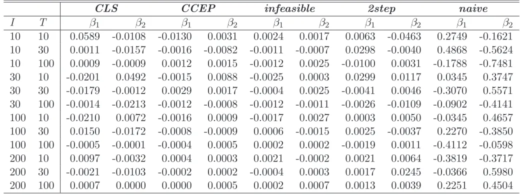
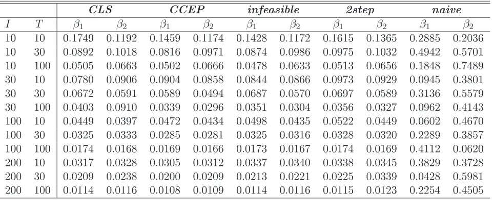
First we compare the estimators ofβ, i.e. the individual specific components coeffi-cients. Tables 1 and 2 report the bias and the root mean squared errors (RMSE) of the two estimators, respectively. Overall, the Pesaran Common Correlated Effects Pooled (CCEP) estimator bias is the closest to the one realized by the infeasible es-timator. Bai estimator and 2step estimator show mixed results. For what concerns the efficiency, as measured by the root mean square error, the Pesaran estimator turns out to the best, while the Bai and the 2step estimators have very close per-formances.
[Tables 1 and 2 here]
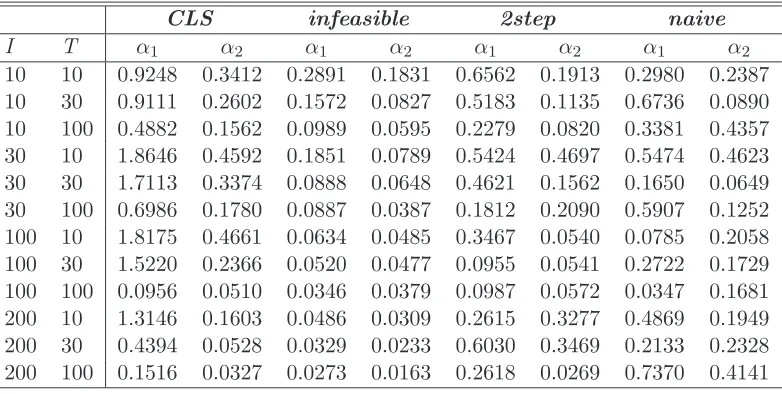
• finite sample properties of α
We now compare the Bai (2005) and the Castagnetti and Rossi (2008) estimator αb
for the common observed components. The two-step estimation method of section 3.2.1 relies on a first-step consistent estimation of the errors eit, which can be used as observed data to obtain consistent (in average norm) estimates of the unobserved factors, ft.
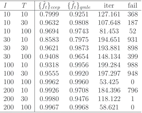
Like in Bai (2003) to evaluate the estimate of a transformation of ft, fbt,2step, we
compute the correlation coefficient between {ft,2ˆstep}Tt=1 and{ft}Tt=1, for each Monte
the results in Bai (2003), obtained in a different context, that is as √T /I → 0, the estimation error in the factor estimates is negligible. It is worth noticing that in many cases the iteration method of Bai (2005) does not converge. The last two columns of table 3 report the average number of iterations and the number of failure for each Monte Carlo simulation, respectively.
[Table 3 here]
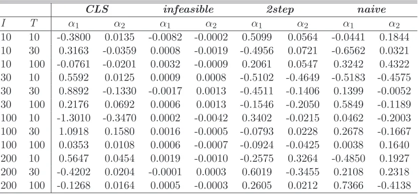
Tables 4 and 5 report the bias and the RMSE of the the Bai (2005) and the two-step estimator of section 3.2.1 estimators of α, respectively. As before we also present estimation results for the naive as well as for the infeasible estimator. For what concerns the bias, when I > T we observe a slightly superior performance of the two-step estimator with respect to the CLS estimator. For the root mean square error we observe a mixed situation. However, we should take into account that the CLS estimator is more computationally intensive than the two-step estimator and that the number of cases in which the iterative procedure fails in achieving the convergence is quite high.
[Tables 4 and 5 here]
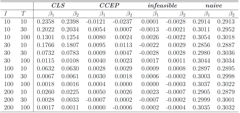
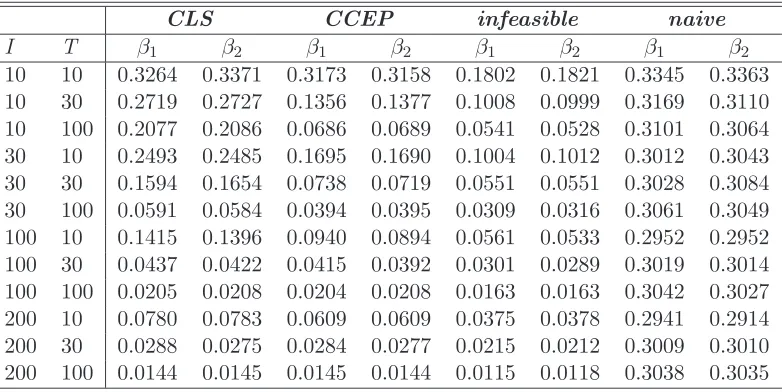
• finite sample properties of β when the factor loadings λi are correlated
with the regressors
Bai (2005) suggests that the method proposed by Pesaran (2006) does not provide consistent estimates of β when λiis correlated with the regressors. Using the pro-jection argument of Mundlak (1978), Bai (2005) suggests that additional regressors, the time-series averages zi= T1ΣTt=1zit where zit = (yit,x
′
it) ′
should also be added to achieve consistency. Appendix 6 shows that the general argument used by Pe-saran (2006) to justify the CCEP estimator holds not only when Ft is correlated with the regressors but also when λiis correlated with the regressors.
Here we investigate the small sample properties of the CCEP estimator when λi is correlated with xit. Following Bai (2005) we adopt the following DGP:
yit=α1d1t+α2d2t+β1x1it+β2x2it+λift+ǫit (20)
x1it =a1+λift+λi+ft+v1it (21)
x2it =a2+λift+λi+ft+v2it (22)
for i= 1, . . . , I, and t = 1, . . . , T. This DGP considers only two individual specific components, x1it and x2it, two observed common factors, d1t and d2t, and one
un-observed common factor ft. ǫit is IIDN(0,2). a = (a1, a2) = (1,1) α= (α1, α2) =
(5,4) and β= (β1, β2) = (1,3).
d1t = 1
d2t = ft+vdt
vdt is IIDN(0,1) independent of all other regressors. The variables λi, ft, vjit are
This DGP is identical to Bai’s (2005) DGP for the case of common regressors. Tables 6 and 7 report the Monte Carlo results in terms of bias and RMSE for β.
[Tables 6 and 7 here]
The Monte Carlo results in table 6 and 7 show that Pesaran (2006) estimator has better bias and root mean square error performances than the Bai estimator when the xit are simultaneously correlated with λi and ft.
5
Conclusions
In this paper we review the estimation techniques adopted in panel data models with individual and common factors. In particular we consider the presence of unobserved and observed common factors. We present also a new approach to the estimation of individual-specific components along with the estimation of the common factors coefficients which is based on a two-step estimation procedure. The finite sample properties are investigated by means of Monte Carlo simulations, under different data-generating processes. The results show that the CCEP estimator by Pesaran (2006) has remarkable properties under different DGPs. Furthermore, the two-step estimator by Castagnetti and Rossi (2008) shows good finite sample properties when compared to the iterative CLS estimator by Bai (2005), which is computationally more demanding and less accurate when we consider the fact that it fails to achieve convergence in a relevant number of cases.
6
Appendix
When the factor loadings are correlated with the regressors, model (1-2) becomes:
yit=β′xit+λi′ft+ǫit (23)
xit =Λi′ft+Aλi+vit (24)
whereΛiis a (r×K) factor loading matrix with fixed components,Λ, andAis a (K×r) matrix of parameters. Combining (23-24) we have the system of equations:
zit=
yit
xit
=Ci′ft+Bλi+uit (25)
where
Ci= λi Λi
1 0
β IK
B=
β′ IK
A
and
uit =
β′vit+ǫit
vit
Consider the cross-section averages of the equations in (25):
¯
zt =C¯′ft+Bλ¯+u¯t (27)
suppose that Rank(C¯) =r≤K+ 1 for all I, then we have:
ft= (C¯C¯
′
)−1C¯(z¯
t−Bλ¯−u¯t) (28)
Pesaran (2006), (Lemma 1) shows that u¯t
q.m.
→ 0 as I → ∞ for every t. Moreover, as in Pesaran (2006), λ¯ →p λas I → ∞ where λ=E(λi) and C¯
p
→C where
C = E(λi) E(Λi)
1 0
β IK
= λ Λ
1 0
β IK
Therefore, from (28) we obtain:
ft−(C¯C¯
′
)−1C¯(z¯
t−Bλ)
p
→0 (29)
References
Ahn, S., Y. Lee, and P. Schmidt (2001): “GMM Estimation of Linear Panel Data Models with Time-varying Individual Effects,”Journal of Econometrics, 101, 219–255. (2006): “Panel Data Models with Multiple Time-Varying Individual Effects,” mimeo.
Ahn, S., and M. Perez(2008): “GMM Estimation of the Number of Latent Factors,” mimeo.
Bai, J. (2003): “Inferential Theory for Factor Models of Large Dimensions,” Economet-rica, 71(1), 135–171.
(2005): “Panel Data Models with Interactive Fixed Effects,” mimeo.
Bai, J., and S. Ng(2002): “Determining the Number of Factors in Approximate Factor Models,” Econometrica, 70(1), 191–221.
(2006a): “Confidence Intervals for Diffusion Index Forecasts and Inference for Factor-Augmented Regressions.,” Econometrica, 74(4), 1133–1150.
(2006b): “Evaluating Latent and Observed Factors in Macroeconomics and Finance.,”Journal of Econometrics, 113(1), 507–537.
Castagnetti, C., and E. Rossi (2008): “Euro Corporates Bonds Risk Factors,” Mimeo.
Coakley, J., A. Fuertes, and R. Smith(2002): “A Principal Component Approach to Cross-Section Dependence in Panels,” Discussion paper, Birkbeck College.
Cochrane, J., andM. Piazzesi(2005): “Bond Risk Premia,”The American Economic Review, 95, 138–160.
Fama, E., and K. French (1993): “Common Risk Factors in the Returns on Stocks and Bonds,” Journal of Financial Economics, 33(1), 3–56.
Kao, C., L. Trapani, and G. Urga(2008): “The Asymptotics for Panel Models with Common Shocks,” mimeo.
Kapetanios, G., and M. Pesaran (2005): Alternative Approaches to Estimation and Inference in Large Multifactor Panels: Small Sample Results with an Application to Modelling of Asset Returnsvol. forthcoming in The Refinement of Econometric Estima-tion and Test Procedures: Finite Sample and Asymptotic Analysis. Garry Phillips and Elias Tzavalis, Cambridge, cambridge university press edn.
Lettau, M., and S. Ludvigson (2001): “Resurrecting the (C)CAPM: A Cross-Sectional Test When Risk Premia are Time Varying,” Journal of Political Economy, 109, 1238–1287.
Ludvigson, S., and S. Ng (2008): “Macro Factors in Bond Risk Premia,”The Review of Financial Studies, forthcoming.
Mardia, K., J. Kent, and J. Bibby (1979): Multivariate Analysis. Academic Press.
Moon, H. R., and M. Weidner (2008): “Asymptotic Analysis of the quasi-MLE of Panel Regression Models with Interactive Fixed Effects,” Department of Economics, UCS.
Mundlak, Y. (1978): “On the Pooling of Time Series and Cross Section Data,” Econo-metrica, 46, 69–85.
Neyman, J., and E. Scott (1948): “Consistent Estimates Based on Partially Consis-tent Observations,” Econometrica, 16, 1–32.
Pesaran, M. (2004): “Estimation and Inference in Large Heterogeneous Panels with a Multifactor Error Structure,” mimeo, Cambridge University.
(2006): “Estimation and Inference in Large Heterogeneous Panels with a Mul-tifactor Error Structure,”Econometrica, 74(4), 967–1012.
Pesaran, M., and R. Smith (1995): “Estimating Long-Run Relationships from Dy-namic Heterogeneous Panels,” Journal of Econometrics, 68(1), 79–113.
Stock, J., and M. Watson (2002): “Macroeconomic Forecasting Using Diffusion In-dexes,” Journal of Business and Economic Statistics, 20, 147–162.
Table 1: BIAS of β estimators
CLS CCEP infeasible 2step naive
I T β1 β2 β1 β2 β1 β2 β1 β2 β1 β2
10 10 0.0589 -0.0108 -0.0130 0.0031 0.0024 0.0017 0.0063 -0.0463 0.2749 -0.1621 10 30 0.0011 -0.0157 -0.0016 -0.0082 -0.0011 -0.0007 0.0298 -0.0040 0.4868 -0.5624 10 100 0.0009 -0.0009 0.0012 0.0015 -0.0012 0.0025 -0.0100 0.0031 -0.1788 -0.7481 30 10 -0.0201 0.0492 -0.0015 0.0088 -0.0025 0.0003 0.0299 0.0117 0.0345 0.3747 30 30 -0.0179 -0.0012 0.0029 0.0017 -0.0004 0.0025 -0.0041 0.0046 -0.3070 0.5571 30 100 -0.0014 -0.0213 -0.0012 -0.0008 -0.0012 -0.0011 -0.0026 -0.0109 -0.0902 -0.4141 100 10 -0.0210 0.0072 -0.0016 0.0009 -0.0017 0.0027 0.0003 0.0050 -0.0345 0.4657 100 30 0.0150 -0.0172 -0.0008 -0.0009 0.0006 -0.0015 0.0025 -0.0037 0.2270 -0.3850 100 100 -0.0005 -0.0001 -0.0004 0.0005 0.0002 0.0002 -0.0019 0.0011 -0.4112 -0.0598 200 10 0.0097 -0.0032 0.0004 0.0003 0.0021 -0.0002 0.0021 0.0064 -0.3819 -0.3717 200 30 -0.0021 -0.0103 -0.0002 0.0002 -0.0004 0.0003 0.0017 0.0245 -0.0366 0.5980 200 100 0.0007 0.0000 0.0000 0.0005 0.0002 0.0007 0.0013 0.0039 0.2251 0.4504
Table 2: RMSE of β estimators
CLS CCEP infeasible 2step naive
I T β1 β2 β1 β2 β1 β2 β1 β2 β1 β2
10 10 0.1749 0.1192 0.1459 0.1174 0.1428 0.1172 0.1615 0.1365 0.2885 0.2036 10 30 0.0892 0.1018 0.0816 0.0971 0.0874 0.0986 0.0975 0.1032 0.4942 0.5701 10 100 0.0505 0.0663 0.0502 0.0666 0.0478 0.0633 0.0513 0.0656 0.1848 0.7489 30 10 0.0780 0.0906 0.0904 0.0858 0.0844 0.0866 0.0973 0.0929 0.0945 0.3801 30 30 0.0672 0.0591 0.0589 0.0494 0.0687 0.0570 0.0697 0.0589 0.3136 0.5579 30 100 0.0403 0.0910 0.0339 0.0296 0.0351 0.0304 0.0356 0.0327 0.0962 0.4143 100 10 0.0449 0.0397 0.0472 0.0434 0.0498 0.0435 0.0522 0.0449 0.0602 0.4670 100 30 0.0325 0.0333 0.0285 0.0281 0.0325 0.0316 0.0328 0.0320 0.2289 0.3857 100 100 0.0174 0.0168 0.0169 0.0166 0.0173 0.0167 0.0174 0.0169 0.4112 0.0620 200 10 0.0317 0.0328 0.0305 0.0312 0.0337 0.0340 0.0338 0.0345 0.3829 0.3728 200 30 0.0209 0.0238 0.0200 0.0209 0.0213 0.0221 0.0225 0.0339 0.0428 0.5981 200 100 0.0114 0.0116 0.0108 0.0109 0.0114 0.0116 0.0115 0.0123 0.2254 0.4505
Table 3: Average correlation coefficients between {fˆt}Tt=1 and {ft}Tt=1.
I T {fˆt}ccep {fˆt}qmle iter fail
10 10 0.7999 0.9251 127.161 368 10 30 0.9632 0.9808 107.648 187 10 100 0.9694 0.9743 81.453 52 30 10 0.8583 0.7975 194.651 931 30 30 0.9621 0.9873 193.881 898 30 100 0.9408 0.9654 148.134 399 100 10 0.9318 0.9956 199.284 988 100 30 0.9555 0.9920 197.297 948 100 100 0.9962 0.9960 53.425 0 200 10 0.9926 0.9708 184.396 796 200 30 0.9980 0.9476 118.122 1 200 100 0.9967 0.9968 58.621 0
Table 4: BIAS of α estimators
CLS infeasible 2step naive
I T α1 α2 α1 α2 α1 α2 α1 α2
10 10 -0.3800 0.0135 -0.0082 -0.0002 0.5099 0.0564 -0.0441 0.1844 10 30 0.3163 -0.0359 0.0008 -0.0019 -0.4956 0.0721 -0.6562 0.0321 10 100 -0.0761 -0.0201 0.0032 -0.0009 0.2061 0.0547 0.3242 0.4322 30 10 0.5592 0.0125 0.0009 0.0008 -0.5102 -0.4649 -0.5183 -0.4575 30 30 0.8892 -0.1330 -0.0017 0.0013 -0.4511 -0.1406 0.1399 -0.0052 30 100 0.2176 0.0692 0.0006 0.0013 -0.1546 -0.2050 0.5849 -0.1189 100 10 -1.3010 -0.3470 0.0002 -0.0042 0.3402 -0.0215 0.0462 -0.2003 100 30 1.0918 0.1580 0.0016 -0.0005 -0.0793 0.0228 0.2678 -0.1667 100 100 0.0353 0.0108 0.0006 -0.0007 -0.0924 -0.0425 0.0038 0.1640 200 10 0.5647 0.0454 0.0019 -0.0010 -0.2575 0.3264 -0.4850 0.1927 200 30 -0.4202 0.0204 -0.0001 0.0003 0.6019 -0.3455 0.2108 0.2318 200 100 -0.1268 0.0164 0.0005 -0.0003 0.2605 0.0212 0.7366 -0.4138
Table 5: RMSE of α estimators
CLS infeasible 2step naive
I T α1 α2 α1 α2 α1 α2 α1 α2
10 10 0.9248 0.3412 0.2891 0.1831 0.6562 0.1913 0.2980 0.2387 10 30 0.9111 0.2602 0.1572 0.0827 0.5183 0.1135 0.6736 0.0890 10 100 0.4882 0.1562 0.0989 0.0595 0.2279 0.0820 0.3381 0.4357 30 10 1.8646 0.4592 0.1851 0.0789 0.5424 0.4697 0.5474 0.4623 30 30 1.7113 0.3374 0.0888 0.0648 0.4621 0.1562 0.1650 0.0649 30 100 0.6986 0.1780 0.0887 0.0387 0.1812 0.2090 0.5907 0.1252 100 10 1.8175 0.4661 0.0634 0.0485 0.3467 0.0540 0.0785 0.2058 100 30 1.5220 0.2366 0.0520 0.0477 0.0955 0.0541 0.2722 0.1729 100 100 0.0956 0.0510 0.0346 0.0379 0.0987 0.0572 0.0347 0.1681 200 10 1.3146 0.1603 0.0486 0.0309 0.2615 0.3277 0.4869 0.1949 200 30 0.4394 0.0528 0.0329 0.0233 0.6030 0.3469 0.2133 0.2328 200 100 0.1516 0.0327 0.0273 0.0163 0.2618 0.0269 0.7370 0.4141
Table 6: BIAS of β estimators
CLS CCEP infeasible naive
I T β1 β2 β1 β2 β1 β2 β1 β2
10 10 0.2358 0.2398 -0.0121 -0.0237 0.0001 -0.0028 0.2914 0.2913 10 30 0.2022 0.2034 0.0054 0.0007 -0.0013 -0.0021 0.3011 0.2952 10 100 0.1301 0.1254 0.0080 0.0024 0.0026 -0.0022 0.3054 0.3018 30 10 0.1766 0.1807 0.0095 0.0113 -0.0022 0.0029 0.2856 0.2887 30 30 0.0732 0.0783 0.0009 0.0047 -0.0028 0.0028 0.2980 0.3036 30 100 0.0115 0.0108 0.0040 0.0023 0.0017 0.0011 0.3044 0.3034 100 10 0.0632 0.0630 0.0028 0.0029 0.0009 0.0008 0.2897 0.2895 100 30 0.0067 0.0061 0.0030 0.0018 0.0006 -0.0002 0.3003 0.2998 100 100 0.0018 0.0016 0.0004 0.0000 0.0000 -0.0003 0.3037 0.3022 200 10 0.0260 0.0225 0.0050 0.0026 0.0023 -0.0007 0.2905 0.2879 200 30 0.0028 0.0033 -0.0007 0.0002 -0.0007 -0.0002 0.2999 0.3001 200 100 0.0017 0.0011 0.0000 -0.0006 0.0002 -0.0004 0.3035 0.3032
Table 7: RMSE of β estimators
CLS CCEP infeasible naive
I T β1 β2 β1 β2 β1 β2 β1 β2
10 10 0.3264 0.3371 0.3173 0.3158 0.1802 0.1821 0.3345 0.3363 10 30 0.2719 0.2727 0.1356 0.1377 0.1008 0.0999 0.3169 0.3110 10 100 0.2077 0.2086 0.0686 0.0689 0.0541 0.0528 0.3101 0.3064 30 10 0.2493 0.2485 0.1695 0.1690 0.1004 0.1012 0.3012 0.3043 30 30 0.1594 0.1654 0.0738 0.0719 0.0551 0.0551 0.3028 0.3084 30 100 0.0591 0.0584 0.0394 0.0395 0.0309 0.0316 0.3061 0.3049 100 10 0.1415 0.1396 0.0940 0.0894 0.0561 0.0533 0.2952 0.2952 100 30 0.0437 0.0422 0.0415 0.0392 0.0301 0.0289 0.3019 0.3014 100 100 0.0205 0.0208 0.0204 0.0208 0.0163 0.0163 0.3042 0.3027 200 10 0.0780 0.0783 0.0609 0.0609 0.0375 0.0378 0.2941 0.2914 200 30 0.0288 0.0275 0.0284 0.0277 0.0215 0.0212 0.3009 0.3010 200 100 0.0144 0.0145 0.0145 0.0144 0.0115 0.0118 0.3038 0.3035