Sequential Monte Carlo Algorithms for Joint Target Tracking
and Classification Using Kinematic Radar Information
Donka Angelova
Lyudmila Mihaylova
Central Laboratory for Parallel Processing
Department of Electrical and Electronic
Bulgarian Academy of Sciences, 25A Acad.
Engineering, University of Bristol
G. Bonchev St, 1113 Sofia, Bulgaria
Woodland Road, Bristol BS8 1UB, UK
[email protected]
[email protected]
Abstract – This paper considers the problem of joint maneuver-ing target trackmaneuver-ing and classification. Based on recently proposed Monte Carlo techniques, a multiple model (MM) particle filter and a mixture Kalman filter (MKF) are designed for two-class identi-fication of air targets: commercial and military aircraft. The clas-sification task is carried out by processing radar measurements only, no class (feature) measurements are used. A speed likelihood function for each class is defined using a priori information about speed constraints. Class-dependent speed likelihoods are calcu-lated through the state estimates of each class-dependent tracker. They are combined with the kinematic measurement likelihoods in order to improve the process of classification. The two designed estimators are compared and evaluated over a rather complex tar-get trajectory. The results are demonstrating the usefulness of the proposed scheme for the incorporation of an additional speed in-formation. Both filters illustrate the opportunity of the particle filtering and MKF to incorporate constraints in a natural way, providing reliable tracking and correct classification.
Keywords: Joint tracking and classification, particle filter,
multi-ple model, maneuvering target tracking, mixture Kalman filtering
1
Introduction
Recently there has been a great interest in the problem of joint target tracking and classification. Actually, the simul-taneous implementation of these two important tasks in the surveillance systems facilitates the situation assessment, re-source allocation and decision-making [1, 2]. Classification (or identification) usually includes target allegiance deter-mination and/or target profile assessment such as vehicle, ship or aircraft type. Target class information could be ob-tained from an electronic support measure (ESM) sensor, friend-and-foe identification system, high resolution radar or other identity sensors. It could be inferred from a tracker, using kinematic measurements only or in a combination with identity sensors. Target type knowledge applied to the tracker can improve tracking performance by the possibility of selecting appropriate target models. Classification infor-mation can assist in correct data association and false tracks elimination in multiple target tracking systems.
Two basic approaches to classification exist based on Bayesian and Dempster-Shafer theories [3, 2, 1]. Challa and Pulford [4] reveal the feedback loop between tracking and identification and introduce the notion of joint track-ing and classification (JTC). They suggest a Bayesian
al-gorithm for JTC using ESM and radar data. The numeri-cal implementation of their algorithm utilizes a grid-based approach. It is well known that the computational effi-ciency of the grid-based algorithms depends on the state vector dimension. In contrast to the grid-based algorithms, the Monte Carlo algorithms are more easily implementable for highly dimensional systems. Feasible implementa-tions of Bayesian JTC via particle filtering are reported in [5, 6, 2, 7]. We have to mention that [5] is one of the first pa-pers devoted to the application of the particle filtering tech-nique to tracking and identification of two closely spaced objects in clutter. Particle filter for tracking and classify-ing multiple targets is proposed in [6] as well. Automatic target recognition is realized by the inclusion of radar cross section measurements into the measurement vector.
The Monte Carlo approach allows for an accurate repre-sentation of joint state and class probability distributions. This is guaranteed by calculating all integrals as accurately as possible [2] and is achieved at the expense of increased computational costs. The highly non-linear relationships between state and class measurements and non-Gaussian noise processes can be easily processed by the particle fil-tering technique. In addition, flight envelope constraints, particularly useful for this task, can be incorporated into the filtering algorithm in a natural and consistent way [8].
In the present paper, motivated by the results reported in [7], we develop two sequential Monte Carlo algorithms: a particle filter and a mixture Kalman filter (MKF) for solv-ing the problem of tracksolv-ing and classifysolv-ing a maneuversolv-ing target using kinematic measurements only. Two air target classes are considered: commercial aircraft (slowly maneu-verable, mainly straight line) and military aircraft (highly maneuverable turns are possible). We should be able to un-derstand which type of aircraft we are observing. In view the fact that both types of aircraft can perform slow ma-neuvers, the recognition can only be achieved during the aircraft’s maneuvers with high speed and acceleration. For this purpose, a bank of two multiple model (MM) class-dependent particle filters is designed and implemented. The novelty of the paper relies also on accounting for two kinds of constraints : both on the acceleration and on the speed. We show that “hard constraints” can be naturally incorpo-rated into the Monte Carlo framework. Two speed like-lihood functions are defined based on a prior information about speed constraints of each class. Such kind of con-straints are incorporated in other approaches for decision making [9]. At each filtering step, the estimated speed from each dependent filter is used to calculate a class-dependent speed likelihood and together with kinematic likelihood both are improving the classification process.
The remaining part of the paper is organized as follows. Section 2 summarizes the Bayesian formulation of the JTC problem according to [2, 7, 10]. Section 3 presents a devel-oped MM particle filter and MKF using both speed and ac-celeration constraints. Simulation results are given in Sec-tion 4, and conclusions generalized in SecSec-tion 5.
2
Bayesian joint target tracking and
classification
Consider the following model of a discrete-time jump Markov system, describing the target dynamics and sensor measurements
xk=F(mk−1)xk−1+G(mk−1)uk−1+B(mk−1)wk−1, (1)
zk =h(mk, xk)+D(mk)vk, k= 1,2, . . . , (2)
wherexk ∈Rnx is the base (continuous) state vector with
transition matrix F, zk ∈ Rnz is the measurement
vec-tor with measurement functionh, anduk ∈ Uis a known
control input. The noise processeswk andvkare
indepen-dent iindepen-dentically distributed (i.i.d.) Gaussian having charac-teristics wk ∼ N(0, Q)andvk ∼ N(0, R), respectively. wk is the random input vector, andvk is the random
mea-surement error vector. All vectors and matrices are as-sumed of appropriate dimensions. The modal (discrete) state mk ∈ S , {1, 2, . . . , s} is a time-homogeneous
first-order Markov chain with transition probabilities
πij ,P r{mk =j|mk−1=i},(i, j∈S) (3)
and initial probability distributionP1(i) , P r{m1=i} for i ∈ S, such that P1(i) ≥ 0, and
Ps
i=1P1(i) = 1. We assume that the target belongs to one of theM classes
c ∈ C whereC = {c1, c2, . . . , cM} represents the set of
the target classes. Generally, the number of the discrete states s = s(c), the initial probability distribution P1c(i) and the transition probability matrixπ = [πij]c, i, j ∈ S
are different for each target class.
The joint state and class is time varying with respect to the state and time invariant with respect to the class [2]. Let
©
Zk, Ykª={zi, yi}:i= 1, . . . , k (4)
be the cumulative set of kinematic (Zk) and class (feature) measurements (Yk) up to timek.
The goal of the joint tracking and classification task is to estimate the statexkand the posterior classification
prob-abilities P¡c|©Zk, Ykª¢, c ∈ C based on all available
measurement information©Zk, Ykª.
If we can construct the posterior joint state-class prob-ability density function (pdf) p¡xk, c|
©
Zk, Ykª¢, then
the posterior classification probabilities can be obtained by marginalization overxk:
P¡c|©Zk, Ykª¢=
Z
xk
p¡xk, c|
©
Zk, Ykª¢dx k. (5)
Suppose that we know the posterior joint state-class pdf
p¡xk−1, c| ©
Zk−1, Yk−1ª¢at time instantk−1. Accord-ing to the Bayesian framework, p¡xk, c|
©
Zk, Ykª¢can
be computed recursively fromp¡xk−1, c| ©
Zk−1, Yk−1ª¢ in two steps – prediction and measurement update [2, 7].
The predicted state-class pdfp¡xk, c|
©
Zk−1, Yk−1ª¢ at timekis given by the equation
p¡xk, c|
©
Zk−1, Yk−1ª¢= (6) Z
xk−1
p(xk|xk−1, c)p ¡
xk−1, c| ©
Zk−1, Yk−1ª¢dxk−1,
where the class- and state-conditioned state prediction pdf
p¡xk |xk−1, c, ©
Zk−1, Yk−1ª¢is obtained from the state transition equation (1)
p¡xk|xk−1, c, ©
Zk−1, Yk−1ª¢= (7)
s(c) X
j=1
p¡xk |xk−1, mk=j,
©
Zk−1, Yk−1ª¢
×P¡mk =j |xk−1, c, ©
Zk−1, Yk−1ª¢=
s(c) X
j=1
p¡xk |xk−1, mk=j,
©
Zk−1, Yk−1ª¢
× s(c) X
l=1
πljP
¡
mk−1=l|c, ©
Zk−1, Yk−1ª¢.
The form of the conditional pdf of the measurements
p({zk, yk} |xk, c) =λ{xk,c}({zk, yk}) (8)
It should be noted that because in our case we don’t have feature measurements, the set{Yk}is replaced in the MM particle filter and in the MKF by the speed estimates from theM classes. Together with a speed envelope which form is given in subsection 3.3, they form a virtual “feature mea-surement”.
When the measurements{zk, yk}arrive, the update step
can be completed
p¡xk, c|
©
Zk, Ykª¢= (9)
λ{xk,c}({zk, yk})p ¡
xk, c|
©
Zk−1, Yk−1ª¢
p({zk, yk} | {Zk−1, Yk−1}) ,
where
p¡{zk, yk} |
©
Zk−1, Yk−1ª¢= (10) X
c∈C
Z
xk
p({zk, yk} |xk, c)p
¡
xk, c|
©
Zk−1, Yk−1ª¢dx
k.
The recursion (6)-(9) begins with the prior density
P{x1, c}, x1∈Rnx, c∈C, which is assumed known.
Using Bayes’ theorem, the posterior probability of the discrete statemk for classcis expressed by
P¡mk =j|c,
©
Zk, Ykª¢= (11)
1 lk
p¡{zk, yk} |mk =j, c,
©
Zk−1, Yk−1ª¢
× s(c) X
l=1
πljP
¡
mk−1=l|c, ©
Zk−1, Yk−1ª¢,
wherelk is a normalizing constant. Eq. (11) is substituted
in (7) in order to predict the state pdf at timek+ 1.
Then the target classification probability is calculated by the equation
P¡c|©Zk, Ykª¢= (12)
p¡{zk, yk} | c,
©
Zk−1, Yk−1ª¢P¡c|©Zk−1, Yk−1ª¢ P
c∈Cp({zk, yk} | c,{Zk−1, Yk−1})P(c| {Zk−1, Yk−1})
with an initial prior target classification probabilityP1(c), P
c∈CP1(c) = 1.
The state estimatexˆckfor each classc
ˆ xc
k=
Z
xk
xkp
¡
xk, c|
©
Zk, Ykª¢dx
k, c∈C (13)
takes part in the calculation of the combined state estimate
ˆ xk=
X
c∈C ˆ xc
kP
¡
c|©Zk, Ykª¢. (14)
It is obvious from (6)-(14) that the estimates, needed for each class, can be calculated independently from the other classes. Therefore, the JTC task can be accomplished by the simultaneous work of M independent filters [11]. The scheme of the particle filter bank, implemented in the present paper is described in Section 3.
3
Maneuvering target tracking and
classification
3.1
Maneuvering target model
The two-dimensional target dynamics is given by
xk =F xk−1+G(uk−1+wk−1), k= 1,2, . . . , (15)
where the state vectorx= (x,x, y,˙ y˙)0 contains target
po-sitions and velocities in the horizontal (Oxy) Cartesian co-ordinate frame. The control input vectoru= (ax, ay)0
in-cludes target accelerations alongxandycoordinates. The process noisew = (wx, wy)0 models perturbations in the
accelerations. The transition matricesFandGare [12]
F =
1 T 0 0 0 1 0 0 0 0 1 T 0 0 0 1
, G=
T2
2 0
T 0
0 T2
2
0 T
, (16)
whereT is the sampling interval andB=G. The target is assumed to belong to one of two classes (M = 2), repre-senting either a lower speed commercial aircraft with lim-ited maneuvering capability (c1) or a highly maneuvering military aircraft (c2) [4]. The flight envelope information comprises speed and acceleration constrains, characteriz-ing each class. The speed v= px˙2+ ˙y2of each class is limited respectively to the interval:
{c1:v∈(100,300)}[m/s] and
{c2:v∈(150,650)} [m/s].
The range of the speed overlap section is
[150,300] [m/s]. The control inputs are restricted to the following sets of accelerations:
{c1:u∈(0,+2g,−2g)} [m/s2] and
{c2:u∈(0,+5g,−5g)} [m/s2],
whereg = 9.81 [m/s2]is the acceleration due to gravity. The acceleration process uk is a Markov chain with five
states (modes)s(c1) =s(c2) = 5[13]:
1.ax= 0, ay= 0 2.ax=A, ay=A
3.ax=A, ay=−A 4.ax=−A, ay=A
5.ax=−A, ay =−A,
whereA= 2gstands for classc1target andA= 5grefers to the classc2. The initial probabilities of the Markov chain are selected as follows: P1(1) = 0.6, P1(2) = P1(3) =
P1(4) = P1(5) = 0.1. The matrixπof transition proba-bilitiesπij, i, j ∈ Sis assumed of the same form for both
types of targets:
π=
0.70 0.10 0.05 0.10 0.05 0.15 0.70 0.05 0.05 0.05 0.15 0.05 0.70 0.05 0.05 0.15 0.05 0.05 0.7 0.05 0.15 0.05 0.05 0.05 0.70
(17)
The standard deviations of the process noise
w ∼ N(0, diag(σ2
mode and class: ©
c1:σjw= 5.5 [m/s2], j= 1, . . . ,5
ª and ©
c2:σ1w= 7.5, σwj = 17.5 [m/s2], j= 2, . . . ,5
ª
,
where (σwx=σwy=σw).
3.2
Measurement model
The measurement model at time k is described by
zk=h(xk) +vk, (18)
where
h(x) =µpx2+y2,arctanx
y
¶0
. (19)
The measurement vector z = (D, β)0 contains the
dis-tance to the target D and bearing β, measured by the radar. The parameters of the measurement error vector
v ∼ N(0, R), R = diag(σ2
D, σ2β)are as follows: σD = 100.0 [m];σβ= 0.15 [deg].
3.3
Speed constraints
Acceleration constraints are imposed on the filter operation by the use of an appropriate control input in the target model. The speed constraints are enforced through the speed likelihood functions. They are constructed based on the speed envelope information (3.1). If we assume that
g1(vck1) =
0.8 if vc1
k ≤100 [m/s] 0.8−κ1(vck1−100) if(100<vck1≤300)
0.1 if vc1
k >300 [m/s]
and
g2(vck2) =
0.1 if vc2
k ≤150 [m/s] 0.1 +κ2(vck2−150) if(150<vck2≤650) 0.95 if vc2
k >650 [m/s]
for κ1 = 0.7/200 and κ2 = 0.85/500, then the class-conditioned speed likelihood functions will have the form, depicted in Fig. 1.
0 100 200 300 400 500 600 700 0
0.1 0.2 0.3 0.4 0.5 0.6 0.7 0.8 0.9 1
Speed interval
gc
(v)
class 1
[image:4.595.92.256.550.675.2]class 2
Fig. 1: Speed likelihood functions
According to the problem formulation, presented in Sec-tion 2, two class-dependent filters work in parallel with
Nc number of particles for each class. At time step k,
each filter gives a state estimate{xˆc
k, c= 1,2}. Let us
as-sume, that the estimated speed from the previous time step, ©
ˆ
vck−1, c= 1,2ª, is a kind of “feature measurement”.
The likelihoodλ{xk,c}({zk, yk})is factorized [2]
λ{xk,c}({zk, yk}) =fxk(zk)gc(y
c
k), (20)
whereykc = ˆvck−1. Practically, the normalized speed like-lihoods represent estimated by the filters speed-based class probabilities. The posterior class probabilities are modified by this additional speed information at each time step k. The inclusion of the speed likelihoods is done after some “warming-up” interval, comprising filter initialization
3.4
Multiple model particle filter algorithm
Assuming two classes of targets (commercial and non commercial), we design a bank of two independent particle filters for each class. Every particle filter is based of multiple models for the unknown target acceleration uk.
The hybrid particle x = {x, m, c} contains then all the necessary information about the target state, mode and class.
The scheme of each particle filter incorporates the steps:
1. Initialization, k= 1.
For class c= 1,2, . . . , M set P(c) =P1(c) * For j= 1, . . . , Nc, sample
n
x(1j)∼p1(x1, c), m(1j)∼ {P1c(m)}sm(=1c) , c(j)=c o
and set k= 2. End forc
2. For c= 1, . . . , M (possibly in parallel) execute * Prediction step
For j= 1, . . . , Nc generate samples m(kj−)1∼ {πc
lm}sm(c=1) for l=m (j)
k−2andc(j)=c
x(kj)=F x(kj−)1+Guk−1(m(kj−)1, c) +Gwk−1,
wk−1∼N(0, Q(m(kj−)1, c)), * Measurement processing step
on receipt of a new measurement{zk, yk}:
Forj= 1, . . . , Nc evaluate the weights Wk(j)=f(zk |xk(j))gc(yck),
wheref(zk|xk(j)) =N(zk;h(x
(j)
k ), R)
andgc(ykc) =gc
¡
ˆ
vck−1¢; calculate
p¡{zk, yk} |c,
©
Zk−1, Yk−1ª¢=PNc
j=1W (j)
k
setL(c) =PNc
j=1W (j)
k
* Selection step
normalize the weights Wk(j)=Wk(j)/PNj=1c Wk(j) resample with replacementNcparticles
(x(kj);j = 1, . . . , Nc)from the set
(x(kl);l= 1, . . . , Nc)according to the weights * Compute updated state estimate and posterior mode probabilities
ˆ xc
k =N1c
PNc
j=1x (j)
k , P(mk=l) =
P
(m(kj)=l,j∈{1,...,Nc}) PNc
j=1m (j)
k
,l= 1, . . . , s(c)
3. Output: Compute posterior class probabilities and combined output estimate
P¡c|©Zk, Ykª¢=PL(c)P(c|{Zk−1,Yk−1})
M
c=1L(c)P(c|{Zk−1,Yk−1}), ˆ
xk =
PM
c=1P ¡
c|©Zk, Ykª¢xˆc k,
4. Setk←−k+ 1and go to step 2.
Actually, there is fusion at two levels: (i) of state estimates and their pdfs with respect to the classes; and (ii) regarding the acceleration grid within each particle filter.
4
The mixture Kalman filter algorithm
The mixture Kalman filter (MKF) [14, 15] is another se-quential Monte Carlo estimation technique which has been successfully applied to different problems in target tracking and digital communications (See e.g. [16]). The MKF is essentially a bank of Kalman filters (KFs) or extended KFs run with Monte Carlo sampling approach. The MKF is de-rived for state-space models in special form, namely condi-tional dynamic linear model, condicondi-tional linear Gaussian model, or partially linear Gaussian model:
(
xk =Fλk−1xk−1+Gλk−1(uk−1+wk−1), zk =Hλkxk+Vλkvk,
(21)
wherewk ∼ N(0,Σw),vk ∼ N(0,Σv)are Gaussian
dis-tributed processes. The term conditional justifies the char-acteristic of these models: they are linear and their formu-lation depends on extra random variables, called latent, de-noted asλ. Then, the Monte Carlo sampling is working in the space of latent variables instead of in the space of the state variables. The matrices Fλ andHλ are known,
as-suming thatλis known. For simplicity, in the sequel we are omitting the subscript λ from the matrices of (21).
Given the indicator variable, the KF provides a sufficient statistical characterization of the system dynamics. The MKF relies on the conditional Gaussian property and uses a marginalization operation in order to improve the efficiency of the sequential Monte Carlo estimation technique.
In our JTC problem the indicator variableλ (correspond-ing tom from the previous sections) takes values from a finite discrete set S , {1, 2, . . . , s(c)} and evolves ac-cording to a Markov chain with transition probabilities (3).
LetKFk(j) ={µk(λ(1:jk)),Σ(λ
(j)
1:k)}denote the sufficient
statistics that characterize the posterior mean and covari-ance matrix of the statexk, conditional on the observations z1:k accumulated up to the time instant k, and indicator
variableλ(1:j)k.
The MKF algorithm [15] which we developed for JTC has the following form:
1. Initialization,k= 1
For classc= 1,2, . . . , M set P(c) =P1(c) * For j = 1, . . . , Nc,
sampleλ(1j)∼ {P1c(λ)}sλ(=1c)
and set KF1(j)={µ1(λ1(j)),Σ(λ(1j))},
where µ1(λ(1j)) = ˆµ1andΣ(λ(1j)) = Σ1 are the mean and covariance of the initial state
x1∼N(ˆµ1,Σ1). Set k= 2. End forc
2. For classc= 1,2, . . . , M execute
Forj= 1, . . . , Nc,
* Forλik−1, i= 1, . . . , s(c) (λik−1,λk−1=i)
• run a KF time update step
(µ(kj|)k−1)i =F µ(j)
k−1|k−1+Guk−1(λ
i k−1, c),
(Σ(kj|)k−1)i=FΣ(j)
k−1|k−1FT+GΣw(λik−1, c)GT,
(zk(j|)k−1)i=h((µ(j) k|k−1)i),
(S(kj))i= (H(j) k )i(Σ
(j)
k|k−1)i(H (j)
k )iT +VΣvVT. • on receipt of a measurementzkcalculate
vvi(j) = f(zk|λik, KFk(−j)1)p(λik|λ(kj−)1), where
f(zk|λik, KF
(j)
k−1) = N(zk; (z (j)
k|k−1)i,(S (j)
k )i),
and
p(λik|λ(kj−)1)is the prior transition probability of the indicator.
• end forλik−1
* Sampleλ(kj)from a setSwith probability, propor-tional tovvi(j), i= 1, . . . , s(c).
LetKFk(j)be the one withλ(kj)=l. * complete the KF iteration
Kk(j|k) = (Σk(j|)k−1)l(H(j) k )lT[(S
(j)
k )l]−1, µ(kj|k) = (µk(j|)k−1)l+K(j)
k|k[zk−(z
(j)
k|k−1)l],
Σ(kj|)k = (Σk(j|)k−1)l−K(j)
k|k(S
(j)
k )lK
(j)T k|k ,
* update the importance weights
Wk(j)=Wk(j−)1gc
¡
ˆ
vkc−1¢ Pis=1(c)vvi(j)
end forj
* Resampling in the same way as in the particle filter: generate a new set of samples with associated weights
* Compute the updated state estimate and posterior class probabilities (as in the particle filter)
End forc
Setk←−k+ 1and go to step 2.
A reasonable choice of the proposal distribution
q(λ(kj+1) |λ1:(jk), KFk(j)) for the indicator variable is its pre-dictive distributionq(λ(kj+1) |λ1:(j)k, KFk(j), zk+1)[14].
5
Simulation results
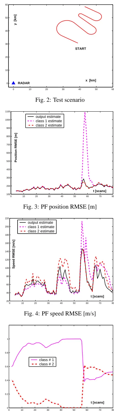
The performance of the implemented filters for JTC is eval-uated by simulations over a representative test trajectory given in Figure 2, together with the radar location, indicated by a triangle. The target motion is generated without pro-cess noise. The MM particle filter and the MKF accounting for speed and acceleration constraints are compared to fil-ters without speed constraints, i.e. which likelihood is com-puted not such as in (20), but is equal toλ{xk,c}=fxk(zk).
Measures of performance. Root-Mean Squared Errors
(RMSEs) [17]: on position (both coordinates combined) and speed (magnitude of the velocity vector), average prob-ability of correct class identification and average time per update are used to evaluate the filters performance. The results presented below are based on 100 Monte Carlo runs. The cloud of the particles for each class is with size Nc = 3000 for the MM particle filter (PF) and Nc = 300for the MKF, whereas the sampling period is T = 5 [s]. The prior class probabilities are chosen as follows: P1(1) = P1(2) = 0.5. The parameters of the base state vector initial distributionx1∼N(x1;m1, P1)in the particle filter algorithm are selected as follows: P1 =
diag{1502 [m], 20.02 [m/s], 1502 [m], 20.02 [m/s]};
m1 contains the exact initial target parameters. The MKF initial parameters are: µˆ1 the mean and the covariance
Σ1 of the initial state x1 ∼ N(ˆµ1,Σ1) are obtained by a two-point differencing technique [12] (p 253). Notice that the noise covariance matrices of the MKF coincide with those of the particle filter, namelyΣv = R,V =I,
Σw=diag{σ2
wx, σ2wy}withσwx=σwy, given in Sec. 3.1
Test trajectory. The target performs four turn maneuvers with intensity1g,2g,5g,2g. The speed is constant, equal to260 [m/s]. After the5gmaneuver, the MM particle filter without speed constraints correctly identifies the real sec-ond class, but after the last maneuver of2g, a tendency for misclassification is present (Figure 5). The MM particle filter with speed constraints correctly determines the class (Figure 6). According to the results from the RMSEs (Fig-ures 3, 4) the developed MM particle filter with accelera-tion and speed constraints can reliably track maneuvering targets.
Nevertheless, as evident from Figures 7 and 12, the filters clearly distinguish different motion segments and provide good estimates of the model probabilities.
It should be mentioned that the selected target model (15) in combination with the particle filtering technique or MKF provides an easy way of imposing acceleration constraints on the target dynamics. Air targets usually perform turn maneuvers with varying accelerations alongxandy coor-dinates. These varying accelerations consecutively make active different models from the designed multiple model configuration, since the models have fixed x- and y- ac-celeration inputs. During maneuvering different models may have similar probabilities which makes difficult to in-fer which is the most probable between them.
0 10 20 30 40 50 60 0
10 20 30 40 50 60
x [km]
y [km]
START
[image:6.595.322.510.53.725.2]RADAR
Fig. 2: Test scenario
0 10 20 30 40 50 60 70 80 100
200 300 400 500 600 700 800 900 1000 1100
t [scans]
Position RMSE [m]
output estimate class 1 estimate class 2 estimate
Fig. 3: PF position RMSE [m]
0 10 20 30 40 50 60 70 80 20
40 60 80 100 120 140 160 180 200 220
t [scans]
Speed RMSE [m/s]
output estimate class 1 estimate class 2 estimate
Fig. 4: PF speed RMSE [m/s]
0 10 20 30 40 50 60 70 80 0
0.2 0.4 0.6 0.8 1
t [scans]
class # 1 class # 2
0 10 20 30 40 50 60 70 80 0
0.2 0.4 0.6 0.8 1
t [scans]
[image:7.595.324.511.57.380.2]class # 1 class # 2
Fig. 6: PF class probabilities (speed constraints)
0 10 20 30 40 50 60 70 80 0
0.2 0.4 0.6 0.8 1
t [scans]
Posterior probability
[image:7.595.84.264.58.205.2]class # 1 class # 2
Fig. 7: PF posterior mode (m=1) probabilities
Figures 8-11 illustrate the performance for the MKF. An important advantage of the MKF compared to the MM par-ticle filter is the smaller peak-dynamic errors during inten-sive maneuvers (with an acceleration5gin the test).
0 10 20 30 40 50 60 70 80 100
150 200 250 300 350
t [scans]
Position RMSE [m]
[image:7.595.83.264.234.387.2]output estimate class 1 estimate class 2 estimate
Fig. 8: MKF position RMSE [m]
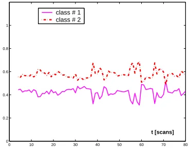
The speed-based class probabilities gc(ˆvc), c = 1,2,
obtained by the MM particle filter and MKF are quite similar. For these reasons we present only the estimated by the MKF functions in Figure 13. The target speed of
260[m/s] provides a slight superiority of the probability, that the target belongs to class 2, according to the speed constraints. The estimated speed probabilities assist in the proper class identification, as we can seen in Figure 11.
0 10 20 30 40 50 60 70 80 20
40 60 80 100 120 140 160 180 200 220
t [scans]
Speed RMSE [m/s]
output estimate class 1 estimate class 2 estimate
Fig. 9: MKF speed RMSE [m/s]
0 10 20 30 40 50 60 70 80 0
0.2 0.4 0.6 0.8 1
t [scans]
class # 1 class # 2
Fig. 10: MKF class probabilities calculated without taking into account speed constraints
0 10 20 30 40 50 60 70 80 0
0.2 0.4 0.6 0.8 1
t [scans]
class # 1 class # 2
Fig. 11: MKF class probabilities calculated using both speed and acceleration constraints
We have to notice that the MM particle filter and MKF com-putational complexity allow for an on-line implementation. An advantage of the MKF is its reduced complexity com-pared to the MM particle filter. The computational time of the PF (withNc= 3000samples) versus the respective one
of the MKF (withNc = 300) is 1.73. We obtained very
good results for the MKF withNc = 200as well. In this
[image:7.595.81.264.489.651.2]0 10 20 30 40 50 60 70 80 0
0.2 0.4 0.6 0.8 1
t [scans]
Posterior probability
[image:8.595.82.266.56.204.2]class # 1 class # 2
Fig. 12: MKF posterior mode (m=3) probabilities
0 10 20 30 40 50 60 70 80 0
0.2 0.4 0.6 0.8 1
t [scans]
class # 1 class # 2
Fig. 13: MKF speed-based class probabilities
6
Conclusions
A Bayesian joint tracking and classification technique has been recently proposed in [2]. It offers the designer a possi-bility of selecting different state spaces and different filter-ing procedures, suitable for each target type. Motivated by this approach, we have designed a multiple model particle filter and a mixture Kalman filter for the purposes of joint maneuvering target tracking and classification and evalu-ated their performance. We have shown that distinct con-straints, enforced by the changeable target behavior can be easily incorporated into the Monte Carlo framework. Two air target classes are considered: commercial and military aircraft. The classification task is accomplished by process-ing kinematic information only, no class (feature) measure-ments are used. For that purpose a bank of two multiple model class-dependent particle filters is designed and im-plemented in the presence of speed and acceleration con-straints. The acceleration constraints for each class are im-posed by using different control inputs in the target model. The speed constraints are enforced by constructing class-dependent speed likelihood functions. Speed likelihoods are calculated at each filtering step and assist in the process of classification. It was shown that speed and acceleration constraints can be accounted for in a similar way in a MKF. The filters performance is analyzed by simulation over typical target trajectory in a plane. The results show a reliable tracking and correct target type classification. A generalization of the algorithms’ application to the three-dimensional case is straightforward.
Acknowledgements.This research is supported by the Bul-garian Foundation for Scientific Investigations under grants I-1202/02 and I-1205/02 and in part by the UK MOD Data and Information Fusion Defence Technology Center.
References
[1] Henry Leung and Jiangfeng Wu. Bayesian and Dempster-Shafer target identification for radar surveillance. IEEE Trans. Aerospace and Electr. Systems, 36(2):432–447, 2000.
[2] Neil Gordon, Simon Maskell, and Thia Kirubarajan. Effi-cient particle filters for joint tracking and classification. In
Proc. SPIE Signal and Data Processing of Small Targets,
volume 4728, Orlando, USA, April 1–5 2002. SPIE.
[3] Alfonso Farina, Pierfrancesco Lombardo, and M. Marsella. Joint tracking and identification algorithms for multisensor data. IEE Proc.-Radar Sonar, Navig., 149(6):271–280, 2002.
[4] Subhash Challa and Graham Pulford. Joint target tracking and classification using radar and ESM sensors. IEEE Trans.
on Aerosp. and Electr. Systems, 37(3):1039–1055, 2001.
[5] David Salmond, David Fisher, and Neil Gordon. Tracking and identification for closely spaced objects in clutter. In
Proc. of the Europ. Contr. Conf., Brussels, Belgium, 1997.
[6] Shawn Herman and Pierre Moulin. A particle filtering ap-propach to FM-band passive radar tracking and automatic target recognition. In IEEE, editor, Proc. of the IEEE
Aerospace Conf., Big Sky, Montana, March 2002. IEEE.
[7] Mahendra Malick, Simon Maskell, Thia Kirubarajan, and Neil Gordon. Littoral tracking using particle filter. In Proc.
of the Fifth Int. Conf. Information Fusion, USA, July 2002.
[8] Subhash Challa and Niclas Bergman. Target tracking in-corporating flight envelope information. In Proc. Third Int.
Conf. Information Fusion, Paris, France, July 2000. ISIF.
[9] Albena Tchamova, Tzvetan Semerdjiev, and Jean Dezert. Estimation of target behaviour tendencies using Dezert-Smarandache theory. In Proc. of the Sixth Intl. Conf. Inform.
Fusion, pages 1349–1356, Australia, July 2003. ISIF.
[10] Arnaud Doucet, Neil Gordon, and Vikram Krishnamurthy. Particle filters for state estimation of jump Markov linear systems. IEEE Trans. on Signal Proc., 49(3):613–624, 2001.
[11] Arnaud Doucet, Nando de Freitas, and Neil Gordon.
Se-quential Monte Carlo Methods in Practice. Springer-Verlag,
New York, USA, 2001.
[12] Yaakov Bar-Shalom and Xiao-Rong Li. Estimation and Tracking: Principles, Techniques, and Software. Artech House, Norwood, MA, 1993.
[13] Amir Averbach, Samuel Itzikowitz, and Tal Kapon. Radar target tracking – Viterbi versus IMM. IEEE Trans. on Aerospace and Electronic Systems, 27(3):550–563, 1991.
[14] Jun S. Liu and Rong Chen. Sequential Monte Carlo methods for dynamic systems. Journal of the American Statistical
Association, 93(443):1032–1044, 1998.
[15] Rong Chen and Jun S. Liu. Mixture Kalman filters. Journal
of the Royal Statistical Society B, (62):493–508, 2000.
[16] Zhe Chen. Bayesian filtering: From Kalman fil-ters to particle filfil-ters, and beyond. Adaptive Syst. Lab., McMaster Univ., Hamilton, ON, Canada. [Online], http://soma.crl.mcmaster.ca/˜zhechen/homepage.htm, 2003.
[image:8.595.81.265.236.381.2]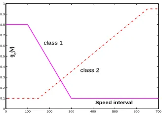
![Fig. 8: MKF position RMSE [m]](https://thumb-us.123doks.com/thumbv2/123dok_us/7990082.759146/7.595.81.264.489.651/fig-mkf-position-rmse-m.webp)