A useful case study on decision making related to financing methods: learning about finance by study case

A useful case study on decision making

related to financing methods: learning

about finance by study case

Voicu, Ionut Cristian and Voicu, Vasilica and Voicu, Andreea

Raluca

June 2008

Online at

https://mpra.ub.uni-muenchen.de/9168/

Being a young graduated student I understood the importance of the

access to information. And how could we become better, unless by

studying already existing know-how?

I know that I am not the best English writer and speaker, but this

book wants to be a pulse for you, the readers, to enhance what you

Ionut Cristian Voicu

LEARNING ABOUT FINANCE BY A

REAL-CASE STUDY

FINANCING METHODS

-- BUDGETING, INCOME ACCOUNTS,

AND BALANCE SHEET FORECASTING

METHODS -

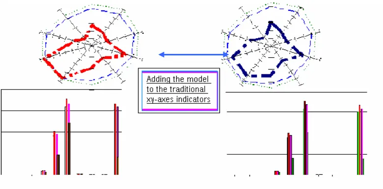
Added-Value: Financial indicators backed by “Circle -

Masterpiece of finance

“Value – the amount of issues giving the item’s price; the money balance of object.”

Resume

The investment value is forecast as being the most probable and achievable value.

The goals of financial management and the preference relating the financing resources have fluctuated historically.

The forecast of performance has to be done step by step upon each element or group of elements.

The future marketing strategy is playing a major role in the sales forecast, while the historical costs are useful when computing the expenses forecast.

The finance, nothing else but the pure research finance, has

studied and explained the process of valuation as a variable of work skills’ interest. When being said “work skills”, it means employees and employers, capital and rent, money and securities. The value of work production is the exchange price. This is nothing else but a weighing scale of needs and expectations. Each businessman has its own scale of importance coefficients for his/her wealth backed by expectations and

economic synergy. As a result of such a financial information-melting

process the economy has evolved to the actual stage of negotiation, disclosure, competition, needs’ satisfaction, and supply vs. offer phenomena. It can with no doubt be said that the impulse of finance is the value of trade, motivation of fighting, the sense of life style. No one can says that he/she knows the secret of fortune, but there are people who dared to get involved into the exchange economy. Thus these operators are able to cover their increasing actual expenses, needs and expectations by the financing instruments (money , securities, gold, land, so on) previously inherited or acquired on

- money market,

- financial market,

or by

- mergers and take-over,

- selling and buying retail/wholesale.

The business partners often have different goals: the seller

was their reference price? Well, the reference price was the computed result of an evaluation methodology more or less scientific, with more or less hypothesis and premises. The science of finance has been developing such evaluation methods raging from those based on cash-flow up to the patrimonial ones. There should be well understood that no sign of equality is between the market price and the computed value. The market price represents the point where offer meets demand in price and quantity, while the computed value is used as a probable price being the result of subjective hypothesis and accepted standards of measurement.

Despite the wide range of financial theories, it is important

not to forget the common elements found among the value‘s definitions:

- the value is seen as the most probable price;

- a free market economy and mechanism are required;

- there are used many terms indicating the target value: market

value, correct value, liquidity value, residual value, net value, investment value, book value, selling value, so on. No matter which terms of value are used, finally all are the result of financial analysis of financing resources.

Financing objectives and resources

The science of finance is a continuous chain of events

looking for different objectives. Depending on the chosen targets there are done various analysis and forecasts on micro- or macroeconomic levels.

Taking as reference point the dynamics of importance of

management perception in area of activity objectives among a portfolio of a certain vector of East European stock-exchange listed companies, a

dissertation study1 on that (East European) country showed the following

dynamics recorded during a 10-years period:

4 . 2 9 4 . 6 1

4 . 0 1 4 . 4 1

3 . 1 8 2 . 9 7

2 . 8 3

4 . 3 8 3 . 0 7

6 . 0 4

N N + 10 Y e ar s

S h a r e h o ld e rs w e a lth ( Y 1 ) E a rn in g p e r s h a r e ( Y 1 ) S a le s (Y 2 ) R e tu rn (Y 2 ) R e v e n u e /I n v e s tm e n t ( Y 1 )

Figure no 1 – Performance management objectives

1

Andreea R. Voicu - Research study included in graduation dissertation, Academy of Economic Studies, Faculty of Finance Insurance Banks and Stock Exchange (Romania), 2005

- the orientation of management toward one or another objective is often more a psychological decision rather than an appraisal analysis. It is necessary a highly motivation self-feed-back control of the decision making process in order to have the best chance to fit the shareholders’ expectation.

Taking in consideration the preferences toward different

financing instruments, there are recorded the following evolutions for a 10-years period:

Shares and bonds (Y1) Banking loans (Y2) Capitalisation (Y2) Alte modalitati (Y1)

N N+1 N+2 N+3 N+4 N+5 N+6 N+7 N+8 N+9

Figure no 2 – Financing instruments

− it shows the effect of a down trend of interest rates on money

market and the effect of increasing role of economic cycles. It’s a momentum when the projects’ financing resources are cheap money for borrower and expensive for the lender. The lower the interests rates, the narrower the spread between banks’ active and passive interests rates, and the higher the pressure on financial markets for cutting expenses.

Related to the management resources’ mix (choice), the

Corporations/companies usually have much more financing needs during and immediately after the economic booms, but their lowest money needs come after the recessions have reached the bottom momentum:

Figure no 3 – Investment money demand

The financing decisions are always under the pressure of a

mix of factories (consisting in business risk, interest risk, market risk, etc.), backed by several vulnerabilities (political and economic weakness, foreign trade dependency, capital flows, regional instability, and so on).

Important recommendations of forecasting methodology

- The step-by-step appraisal of forecast means improvement of

existing links between independent variables with the dependent ones.

- The process of data collection and interpretation generates a lot

of residual influences (i.e. influences from the human expectations upon the working capital structure, profitability, average periods, sales and revenue, costs and trends). Thus the analysis and methodology have to consider as being useful to adopting a pessimistic variant doubled by an optimistic one as action of response to the subjective chosen hypothesis. But if there is no time for such laborious work, the analysts could adopt just one medium optimistic analyses (if there is a boom period), or medium pessimistic one (if there is a recession).

- The forecast period has to be fit according to the each company

correlations on the labor policy, investment trends, production equipment regeneration, loans and repayments, maturity, acquisitions, and expenses vs. revenue.

- The main elements of the capital are considered to be the

equity, legal reserves, retained profits, long term financing loans.

Sales forecast

- Such effort comes firstly with a marketing plan about

economic potential, market share, suppliers and distribution channels, market dispersion, etc. There are issued hypothesis/ premises upon the offer and supply, potential and perspectives, subsides and facilities, financial products’ history. The actual researches in these areas are trying to explain the phenomenon by financial and quantitative methods, and by mathematics links. There are widely used mobile averages, auto reversibility, white noise concepts, lags, differences, correlation degree, so on. The forecasting base is represented by the amount of sales being the reference point of the other dependent variables: salaries, raw material, operating costs, inventory, receivables, administration level, cash and current loans, financial/non financial long terms loans.

Expenses forecast

The analysis cares the structure of expenses being items

which values could increase/decrease at a higher rate (i.e. -/+ 5%) than the sales value rate. Several linear econometric models of first degree are likely to look as the followings:

Item value(y) = A * Sales(x),

Item value(y)=A * Sales(x) + Constant

all coefficients are computed on a financial base, usually being used the 1000 monetary units revenue’s proportion related to the chosen premises and strategic goals, macroeconomics practice, competition, so on.

By its specific characteristics the financial forecast uses

About the working hypothesis their utility consists in the

subjective evolutions on the company and economy trends as a result of previously taken decisions of management with direct effect on forecasting behavior. One important example is given by externalities – these are external effects not due to the added value but to the favorable conjuncture in resources allocation. Such positive or negative effects could be often generated. Thus a necessary condition is to balance the expectation with the possibility of production and solving financial crises.

Depending on the degree of representative level, the

following methods are used by the analysts :

- probability methods – known changing variables, known

happening probability, expected variance;

- uncertainty methods – unknown changing variables, unknown

variance;

- certainty methods – known changing variables, known

variance and evolution.

Notes

Evaluation methods Exchange price Financing instruments Financing needs Financing objectives Forecast methodology

Goals

Investment climate Resources

Statistics and geometrical design as tools of

the risk and performance analysis

Resume

Quantitative statistics models come to reveal the risk measure.

Time interval analysis should cover at least 2-3 years of continuous activity.

The limitation of chosen financial indicators comes from the data disclosure availability and working principles.

The objective is a lower risk of adopting a wrong financing strategy. The financial indicators should be enhanced by a circle view graphic for a better fitting of conclusions and observations. That methodology supposes an allocation of one graphic axe to each chosen indicator.

The overall performance is represented by the geometrical surface resulting from the correlations and juncture of activity variables.

The financial economy’s environment has as result a strong

association of money market variables. This point of view has its arguments arising especially from the effects of investment climate and lending behavior. By the new modern analysis techniques, the participants (borrowers and lenders) are involved in the process both as the financial analysts and also as the analyzed subjects/objects. All these arguments gathering into a great competition will have the solution for achieving a higher performance among the contractual parts.

According to the spirit of mathematics existing among all

researchers, each financial analyst (senior or junior experience) must be able to apply quantitative statistics developed by the software companies so having the capacity of description the economic links among chosen variables. The linear or nonlinear models born by such studies will finally mean more than just the objectives, they will come to reveal the economy and to describe the risk measures.

Round-view financial analysis

My professional experience acquired on the banking area

additional analysis in time and space. It implies the use of working principles and procedures, establishment of objectives – all these coming to be an image of each individual experience and expectations.

Modeling the series of financial indicators

Working principles

The applied methodology is set on a research done upon a

database of reported indicators of Stock Exchange Listed Companies (having market value due to the listing acceptance’s procedures), and which is related to the individual financial performances of chosen company.

The working principles can be noticed as it follows:

A. Performance’s interpretation is improved by a graphical

representation, without any relation to any standard indicator other than the database of finance-statistics investigation.

B. The analysis requires representative aspects consist of: net profit

and a continuous activity for at least 2-3 years, information transparency, professional management and accountability competence, market capitalization, acceptable liquidity, and low activity volatility.

C. The limitation of chosen financial indicators comes only from the availability of data disclosure, being obtained the following proposed default matrix that can be increased or decreased in axes number:

X1 - Gross Profit / Asset X2 – Liabilities / Net worth X3 – Sales / Assets

X4 – EBIT / Interests

X5 – Self Financing / Liabilities X6 – Average Payment Period X7 - Quick ratio

X8 - Current ratio

X9 – Net Profit / Net wealth X10 - Gross Profit / Sales X11 - Net worth /Assets

- there can be more or less than eleven independent variables according to each user’s needs and data availability.

D. The model has the goal to verify the cases when the maximization

of covered surface is obtained.

E. The analysis requires an allocation of one graphic axe to each

chosen indicator, and line connection of indicators’ computed values for each financing method and yearly financial exercise.

F. The methodology has applicability upon the different sizes of

companies (small, medium, or consolidated balances). The importance is that their assets and liabilities dimensions, property form, and Stock Exchange listing acceptance of the studied subjects do not matter (the applicability is ranging from small companies to the big ones).

Objectives

The main objectives of such application are:

1. Obtaining of a dual methodology for a “high velocity” visual

diagnostic test of borrowed customers;

2. Analysis under conditions of real time changes for liquidity,

solvability, profitability, gearing, and so on;

3. Disclosure of weakness and strengthen of the financing plans.

There is a high opportunity to focus exactly on the required aspects;

4. A lower number of wrong financing decisions;

6. New and useful database for all involved analysts.

Working procedures

The brief description of procedures will touch the

following aspects:

a. The geometrical picture will assign one axe to each statistical

analyzed variable in order to disclosure the company’s performances;

b. The representation of computed values for the chosen variables;

c. The establishment of activity risk in terms of minimum surface

accepted;

d. The joined-axes representation - in order to watch for the

interested goals of financial analysis (maximization of surface means better operational performance);

e. The choice of a time interval;

f. The correlation analysis between financial indicators and the

financing methods according to the “round view” interpretation.

A previously described analysis done by “circle view”

procedural methods, would show the following operational advantages:

- Improve of decision making;

- Simplifying and easiness of data interpretation;

- Disclosure of borrowers’ weak-strong points;

- Reliable comparative process using accepted indicators;

- Dynamic approach of individual financial performance;

- Comparable indicators having different unit scale;

- A higher certitude of financial analysis.

Notes

Econometric model Market variable Objectives

Operational advantages Performances

Procedures

Risk measure Round-view chart Significance coefficient Stock Exchange regulations Variables

Case study

Resum

e

The external macroeconomic variables like investment climate and inflation have a high influence on management strategies.

The overall activity analysis implies a disclosure of shareholders history, employment policy, building infrastructure ecology, domestic and foreign market competitions, performance of the last two years activity,

investment strategies, cash flow influences, expenses and revenue forecast.

Each financing method has its own influences on the balance sheet and profitability accounts.

The working principles and hypothesis are not altered by the financing decisions.

The analysis should cover a historic period of at least 2 years, and a forecasting period of 4 to 5 years seen as a minimum pay-back time interval of investment.

The circle view analysis is used to justify and enhance financing decisions.

Pointing the truth

Like any other decisions making area, financial decision is

nothing else but a choice between many possible actions. In the contemporary world, all good decisions are subjects of the following analytic process:

a. Defining the objectives

-the making decision persons should know that the direction of their action has a final purpose. Thus, in the case of an unknown desired destination, the managers have no possibility for choosing the right action way. Among them, the most important objective often chosen is the maximization of shareholders wealth.

b. Financing cost

circumstances the human error in the data process is unavoidable, and the importance of a competitive managerial team comes as a necessity. Financial policy should be the result of a decisional analysis between effect vs. effort, necessity vs. available assets. So, the present part of the book will come with a study done upon several possible financing resources, together with their characteristics and implications.

Irrespective of the company’s option of financing method

of its activity, the management has to be aware that a great influence comes from the global investment behavior. Another influence is the inflation - almost as important as the first one, because it can make an orientation of investor toward other financial or money instruments. Usually the investors use more than one money resource, so it is important for them to know what is the weighted average cost of capital:

WACC=

Σ

Σ

Σ

Σ

C

*p

- where pi is the participation percent for each resource, and Ci is

the cost measure of that resource.

Previously identified elements (subjects) have to be well

understood and represent an important chapter of the investment risk analysis. The analysts’ team has to carry out programs and tasks built for longer and longer periods of time. The perspective of economic problems can be identified at both the microeconomics levels coming from the velocity of structural changes, and macroeconomics levels.

A.

ACTIVITY ANALYSIS OF ARCCRA S.A. COMPANY

(at least 2-3 years period)2

1. Overall information, short-time history

Description: XYZABC SA is a public trade company,

registered at the Chamber (Office) of Trade under number (!?!)……

located in (!?!)…… street ……phone-fax (!?!)………...

Issued shares being worth M_U 66,545,250 thousand (the

chosen measure unit is M_U as the intention was to increase the difficulty degree due to the necessity of forward exchange rate

analysis), divided into a number of 2,661,850 shares with a nominal

(face) value of M_U 25,000. The company has the fiscal address in the

region of (!?!) …….., account number (!?!)……., the regular client

business bank is XXXE-Commercial Bank.

Its main activity objectives according to the statute is the production and trade for the alcoholic and non-alcoholic drinks, dregs, transportation of goods, import-export activity and other different services.

There are about 1,629 employees, structured as following:

- executive management team 3 - execution workers 180 - high skill workers 1,446

The company was established in 1881 by

(!?!)

1909 it became a closed company and in 1948 there was a take-over by

(!?!)

merged with

(!?!)

The main financial data disclosure for the last 3 years of

activity:

Table no1 (M_U thousand )

Specificity 2003 2004 2005

Revenue 8,272,840 20,220,706 39,508,217

Expenses 7,865,814 19,583,370 39,036,712

EBT 407,026 567,207 514,480

Borrowings 1,660,550 2,801,466 10,139,996

Dividends 89,606 124,846 9,035

Long term assets 10,438,217 10,505,057 68,724,879

Depreciation 596,620 1,011,492 952,869

2. Employees approach

The legal labor contracts for 2005 are negotiated between

the company management and the two existing syndicates (!?!): - ARCCRA Syndicate

- ARCCRA’ ISDW (Independent Syndicate of Workers )

The individual labour contracts are establishing

(!?!)…..limits on the wages and bonus depending on the efficiency, experience and high skilled work. The obligations toward community budget have been delayed due to the lack of money flow in the banking account at the maturity of the last year exercise, and that incident has generated legal penalties (!?!)….of M_U 260,528 thousand in 2005.

The executive management is structured into:

o President

o Economic manager

3.Pollution and environment

ARCCRA S.A. has been equipped with a modern

bio-mechanical nonpolluting plant with a capacity of 171 litters/sec since

1987. The Law of Waters no. (!?!) … and the law no…… have been a constant concern of the management, in order to obtain a higher

protection against pollution factors (!?!)….. Thus, the technological

products are used to obtain animal food, huge quantities of Plastic-Fluoride…., or even raw for thermo- or electric power stations.

The company possesses all necessary legal approvals (!?!)

….. for his plants from the environment authorities.

4. Infrastructure

The legal documents indicate an operational land surface as

following:

- total surface(st) 95,235 sqm

- building surface(sc) 33,640 sqm

- road surface(str) 44,504 sqm

- network surface(sr) 6,461 sqm

- free surface(si) 10,630 sqm

- build unfolded surface (sd) 52,800 sqm

The quantity index , the percent of using land is:

POT= (sc+str+sr)/st = 88,84 %

The quality index, the coefficient of unfold land is:

CUT= (sd+str+sr)/sr = 1,09

5. The marketing of products

The analysis of present stage of world economy leads (!?!)

….. at the conclusion that the countries/country have/has gone through an

economic recession/ boom (?!). The beginning of the economic boom

premises for them is set to have happened in …….. The world market of alcoholic drinks is a (?!) monopoly/non monopoly-type market of global acting companies like:

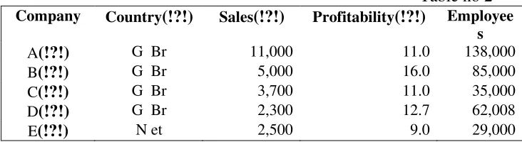
Table no 2

Company Country(!?!) Sales(!?!) Profitability(!?!) Employee s

A(!?!) G Br 11,000 11.0 138,000

B(!?!) G Br 5,000 16.0 85,000

C(!?!) G Br 3,700 11.0 35,000

D(!?!) G Br 2,300 12.7 62,008

F(!?!) G Br 2,900 32.0 19,000

G(!?!) F ra 2,400 29.0 14,000

H(!?!) D en 1,100 9.0 12,008

I(!?!) G Br 1,100 20.0 30,000

The company’s value of exports (!?!) …has been around

USD 3,200,800, obtaining an average price of 1.61 $/litter, below the average price of the other producers and at the limit of manufacturing costs in 2005. The export percentage in the overall production was about 8%. For avoiding any export losses due to forecasted incoming high costs, our firm has to change its actual plants(!?!) …. with others more efficient.

The domestic market has a shares’ coverage (!?!) ….

coming from six important companies including our company.

6. Economic and financial results for 2005 and 2006(four months)

• Analysis of balance sheet.

• Analysis of profit and loss account

Pointing the financial information

The methodology is based on the correlation existing

between the assets, liabilities and shareholders wealth. For the first four months of 2005, there has been an increase in the receivable with bad effects upon the company’s independence, because the investment

program is more dependent on the new financing resources. A higher

attention is imposed to the juridical department for retrieving this

elements. A good sign comes from a low rate of leverage, which means a possible future increase in debts. There has to be noticed a production

program that is set for meeting new market requirements. The value of

overall revenue in 2005 is M_U 39,508,217 thousand (of which the operating sales are about M_U 38,520,479 thousand).

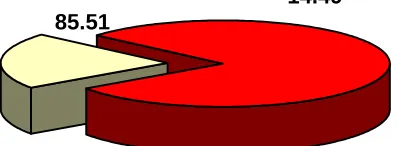
Structure for company’s balance sheet is presented in the next graphic:

Current assets Long term assets

85.51

14.49

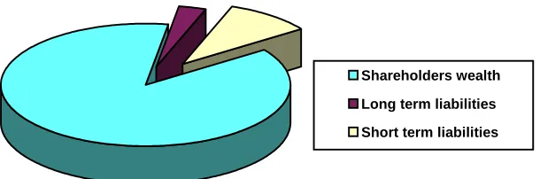
Shareholders wealth Long term liabilities Short term liabilities

9 2

8

Figure no 6 – Structure of resources

The company’s potential capacity of production has not

been fully used due to a conjunctural decrease in the sales that has

determined both lower profit and lower revenue.

About the expenses (it can be noticed) they are at a level of

M_U 988 for every M_U 1000 revenue, leading to a small profit. In 2006 for the first four months, the company recorded M_U 1,314,053 thousand loses but there is forecasted a profit by the end of the year. Considering a number of 1,629 employees for 2005, there results a labour productivity of M_U 24,253 thousand per worker, and for the present year it climbs at M_U 29,667 thousand per worker (almost 20% higher).

Analyzing financial indicators

Using the indicators obtained by the conversion of data in

the balance sheet for 2005 and 2006, it can be seen a little increase in the assets value from M_U 80,371,054 thousand to M_U 80,525,181 thousand.

The proportion of long term assets into total assets has

been facing with a decrease from 85.51% to 85.17%, which in absolute value represents M_U 142,748 thousand. About the current assets, they have known an increase from 14.49% to 14.83% in 2006, which was M_U 11,943,050 thousand (including consolidated accounts). But there is still

maintained a warning signal related to the company’s capacity of

adapting to the possible market changes. It is recommended under these conditions a higher level for the raw materials and their use. Besides, the inventories have a proportion in the current assets of 53.66% in 2005 and 53.99% in 2006, while receivable arrives at 26.53%, respectively 23.42%.

Cash of M_U 721,294 thousand (6.79% of current assets

Regarding to the required funds for investments, the

financing by internal capital has been reduced to 85.23% (in 2006) as

compared to 87.25% (in 2005). The percent of borrowed money in the overall resources arrives at 14.77% from 12.75% in 2005 (funds due to be paid in a period more than one year 2.95%) having a good structure.

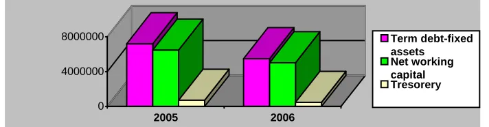
The difference between long term resources and fixed

assets has a downtrend from M_U 7,195,870 thousand to M_U 5,485,408 thousand, being the result either of the continuous reduce of “permanent” funds or the increased fixed assets. The ratio of the previous value divided by the current assets has been lowered for the 2006’s first term at 45.93% from 61.8%. The number of participation for this value to the revenue has recorded an uptrend from 5.5 (times) to 8.65 (times) in 2006.

Net working capital (using the formula: inventory +

receivable - current liabilities), has been reduced with almost M_U 1,459,751 thousand. The effect is a lower cash flow at the first disposal (demand). Thus the company is borrowing on short term the notes of M_U 2,857,774 thousand in 2006.

0 4000000 8000000

2005 2006

Term debt-fixed assets

Net working capital Tresorery

Figure no 7 – Histogram of indicators

The current assets’ financing has been done by its own

funds in a proportion of 32.4% in 2005 and 20.27% for present year. Consequently, there is an increase in the external resources from 38.2% up to 54.0%.

The following part is going to cover the appraisal of

liquidity indicators as a measure of company’s ability for repayment of its

current debts. The current ratio indicates a little difficulty in paying its

debts. The quick assets ratio of the company for this period is consider unsatisfactory and there is a business risk (0.5 in 2005 and 0.37 in 2006). The presence of fixed assets in the total assets value has a constant level of 0.85 for both 2005 and 30 April 2006.

It can be pointed a reducing percent of the company

capacity of coverage for resources by own capital at almost 85.23. That means the company has a low ratio of obligation and a high possibility of financial autonomy. There seems no problem for meeting its long term obligation as it is shown by the overall ratio of debts.

A satisfactory level of debts (for this industry type of

wealth. The ratio of debt to total own equity shows the reliable behaviour of management policy by the levels recorded at 0.14 in 2005 and 0.16 in next year, being inside the optimum interval.

The analysis is to continue with the profitability ratio.

The first four months period of 2006 records a loss of M_U 1,314,053 thousand, but the firm performance has to be related to the profit of the last year (because actual financial exercise has not been finished), having the followings:

• net profit margin computed as ratio between net profit and

total revenue is 0.61%;

• return on equity calculated as report of net profit vs. net worth

is 0.34%;

• the economic profitability obtained by dividing the global

earnings by long term resources is 0.71%;

• earnings per equity is 0.36%;

• gross profit margin is 1.3%.

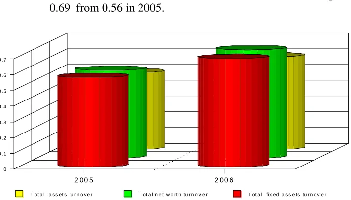
The fixed assets turnover calculated as ratio of annual

sales divided by net fixed assets has a value of 0.69 in 2006 and 0.57 in 2005. Under the hypothesis of maintaining the employees number and a time-period’s extrapolation of statement data up to December 31-th 2006, there can be deduced a higher productivity per employee due to a bonus rewarding policy.

The participation (rotation) rate (degrees of use) for

balance sheet components is improved and the premises are:

1. the total assets turnover jumps from 0.49 to 0.59 in 2006;

2. the current assets turnover swings from 3.39 to 3.97;

3. an increase in the period of average inventory with 1 day;

4. the total shareholders’ wealth turnover has increased up to

0.69 from 0.56 in 2005.

T ot a l a ss et s tu r n o ve r T ot a l n e t w o r t h tu r n o v e r T ot a l fix ed a ss e ts tu r n o v e r

2 00 5 2 00 6

0 0 .1 0 .2 0 .3 0 .4 0 .5 0 .6 0 .7

The previous ratios have disclosed a low profit’s management policy that is an adaptation to the overall economic climate pressure. In 2005 year, there was recorded an operating profit of M_U 1,756,010 thousand (operating revenue - operating expenses) backed by a financial loss of M_U 988,253 thousand (financial revenue - financial expenses) and an exceptional loss of M_U 296,252 thousand (non regular revenue – non regular expenses, e.g. law penalties, commercial penalties). It was preferred such a subjective structure of profit and loss account in

order to pinpoint the influences of those elements being other than

regular revenue and expenses. If you want, you could compute the statement according to your own standards in order to bring it at a standard structure.

B. FINANCIAL AND STRATEGIC PLANNING

years period)3

The company’s strategy

In order to maintain the actual production capacity, the

management has been analyzing several investment financial plans for the last years. So, this approach is to deal with analysis of opportunity of the manufacturing works’ replacements in several production departments.

The CEO board under the request’s influence of

production and marketing advisers has decided the acquisition of two modern plants. The step-by-step opportunity cost analysis among the different plant manufacturers’ offers has generated a winner - K&HMas of G(xxxx), being the most suitable on both technical and economical features and criteria, and an agreement/buying contract has been signed.

There is expected to request an investment of about FRG 14,606,811

(FRG = Foreign Monetary Units), being an equivalent of M_U 6,865.00 million at an exchange rate of M_U/ FRG 470.

For financing this investment, a choice has to be done on a

mixture of possible resources.

Before any further actions, it is ought to perform a

forecasting analysis upon the company’s future financial performances. It

usually starts with those revenue and expenses not influenced by the

chosen methods of financing the accrued payments:

Not Influenced Revenue Forecast

Name 2006 2007 2008 2009 2010 2011

Production sales4

66,933.40 70,449.90 74,163.00 78,266.10 82,165.50 86,615.50 Goods sales 43.50 97.00 194.00 388.00 776.00 1,542.00 Total sales 66,976.90 70,546.90 74,357.00 78,654.10 82,941.50 88,157.50 Stocks’

cash dividend

283.00 283.00 283.00 283.00 283.00 283.00

Adjusted financial revenue

1,252.50 1,319.20 1,390.50 1,470.80 1,551.00 1,648.50

Total financial revenue

1,535.50 1,602.20 1,673.50 1,753.80 1,834.00 1,931.50

Other operating revenue

0.00 0.00 0.00 0.00 0.00 0.00

Overall revenue

68,512.40 72,149.10 76,030.50 80,407.90 84,775.00 90,089.00

It is worth to point out that the production sales’ forecast is

considered the result of an increased production capacity and not as an

inflationary jump of prices. In 2005, the company has not obtained any

goods sales revenue, but since 2006 this activity has brought receipts

being worth at least M_U 43,527 thousand, the management intending to develop and multiply its value twice on each following year. About the

participation income (cash dividends), the company has been holding a

shares portfolio of equivalent M_U 500 million par value at several banks that makes an yearly inflow of almost M_U 283 million. Also, it

received favorable revenues of exchange rates (M_U 654.77 million)

and interests (M_U 24.6 million) in 2005, being considered to get a future fixed amount of 1.87% of net sales (as doing now).

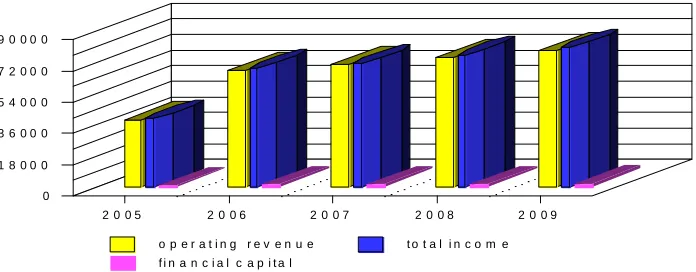
The forecasted operating revenue is characterized by:

• The capital swing is in constant prices;

• The increasing productions compared to the one on 2005 year

are to be the result of higher number of products offered and sold to the customers.

• It is estimated a higher quantity of goods trade

o p e r a t i n g r e v e n u e t o t a l i n c o m e f i n a n c i a l c a p i t a l

2 0 0 5 2 0 0 6 2 0 0 7 2 0 0 8 2 0 0 9 0

1 8 0 0 0 3 6 0 0 0 5 4 0 0 0 7 2 0 0 0 9 0 0 0 0

Figure no 9 – Dynamic structure of income

Not Influenced Expenses Forecast

This procedure is set on the base principle according to

which the investment does not produce any important changes in the structure of expenses because:

• it generates the replacement of the old production plants

• the marginal productivity and quality are going to be noticed in

the supplemental operating income.

It is recommended to be used the forecasting method of

the expenses for each M_U one thousand (1000) operating revenue. The expenses are divided in two categories: fixed and variable. Variable expenses are those being direct influenced by the sales amount according to an index, while the fixed expenses are in opposition with the variable ones on the index terms.

The working hypothesis based on market information: the

expenses are going to increase after 2006 by an index equal to 0.95 of the sales growth:

Table no 4

Specification 2005

M_U mill.

Expenses at M_U 1000

income

Fixed expenses

Variable expenses

Cost of raw materials 9,682.40 251.40 0.00 251.40 Cost of needed

materials

3,048.30 79.10 39.60 39.50

Energy and water 2,168.30 56.30 8.30 48.00

Other cost of materials 2,659.50 69.00 69.00 0.00 Total raw materials 17,588.50 455.80 116.90 338.90

Services 1,139.00 29.60 29.60 0.00

Fiscal taxes 12,620.60 327.60 0.00 327.60

Employee wages 3,405.20 88.40 35.40 53.00

Ancillary social costs 1,085.20 28.20 11.20 17.00 Total employees

outlays

4,490.40 116.60 46.60 70.00

Other operating amounts

Depreciation 952.90 24.80 24.80 0.00 Total operating outlay 36,761.70 954.40 217.90 736.50

The proportion of these outlay in the overall amount for

2005 is:

Figure no 10 – Expenses structure

The depreciation is valued separately being the result of

accountant method and fixed assets evolution. The amount of depreciation in 2005 was M_U 952.9 million maintaining the same value for the present year - 2006, and starting with 2007 it is expected to grow with a supplementary amount of M_U 569.81 million due to:

- Investment= FRG 14,606,811 * M_U/FRG 470 = 6,865.20 (M_U million)

- Duration of use (tool life) = 12 (years) - Depreciation percent = 8.3%

- Annual depreciation = 6,865.20mil * 8.3% = 569.81 (M_U million)

- resulting a future annual total depreciation expense of

M_U 569.81+952.9 (= 1,522.71) million. The forecast computed evolution for the operating outlay is going to be:

Table no 5 ( M_U Million )

Name 2006 2007 2008 2009 2010

Goods expenses 33.00 73.70 147.40 294.90 589.80

Raw materials 16,794.10 17,668.30 18,551.80 19,516.50 20,433.80 Needed materials 2,650.60

2,643.90 2,650.60 2,776.00 2,650.60 2,914.90 2,650.60 3,066.40 2,650.60 3,374.30 Energy and water 555.50

3,212.80 555.50 3,373.40 555.55 3,542.10 555.50 3,726.30 555.50 4,100.40

Other claims 4,618.40 4,618.40 4,618.40 4,618.40 4,618.40

Total raw

materials 30,508.30 31,642.20 32,833.40 34,133.70 35,733.00

Services 1,981.20 1,981.20 1,981.20 1,981.20 1,981.20

Taxes and fiscal obligation

21,927.40 23,023.70 24,174.90 25,432.00 26,627.40

Employees expenses 2,369.40 3,547.50 2,369.40 3,724.90 2,369.40 3,911.10 2,369.40 4,114.50 2,368.40 4,307.60 Social protection expenses 749.70 1,137.80 749.70 1,194.70 749.70 1,254.40 749.70 1,319.70 749.70 1,381.20 Total employees

outlay 7,804.40 8,038.70 8,284.60 8,553.30 8,806.90

Depreciation 952.90 1,522.71 1,522.71 1,522.71 1,522.71

Total operating

expenses 63,174.20 66,208.51 68,796.81 71,622.91 74,671.21

Using previous table, compared to 2005 year, it can be said

that the forecast outlay for each M_U 1000 of revenue is lower with 5.4% than a regular one and there is no other possibility of reduction because the main proportion is held by the variable claims that has a low probability of going down.

The following paragraphs are dealing with the followings:

• the raw material supplying system requires borrowings (from

suppliers or banks);

• the interest paid in 2005 was M_U 50.6 ( = M_U 1,952,528 /

M_U 38,520,479) for every M_U 1000 operating income;

• in 2005 the loans offered to its customers had a period of

repayment of 14.7 days and the liquidity was M_U 721,300 million;

• the current loan interests are going to be no more than M_U 18.9 for every M_U (1000) one thousand.

Related to the previous analysis which has treated

the financial situation of the chosen company, it worth to get a focus upon the appropriate behavior into a choosing process for financing resources on long terms:

Fixed cost

1. BORROWING MONEY FROM BANKS

2. BONDS ISSUE

3. NEW SHARES / RIGHTS ISSUE

4. LEASING CONTRACTS

5. RETAINED PROFIT AND DEPRECIATION

The calculus for each financial strategy has to be linked to the investment requirement coming from the replacement of old production line with a new plant having a value of FRG 14,606,811.

BORROWING MONEY FROM BANK AND SUPPLIER

The following analyzed elements are acting upon the

company (the present economic performance):

1. A downtrend on financing by its internal resources;

2. An increasing proportion of external capital resources

participation;

3. A downtrend in the assets coverage by the difference

between long term resources minus fixed assets;

4. An increased participation for all assets and resources to operating results;

5. A reducing net working assets;

+ all the other conclusions coming from the previous chapter analysis on the company management.

As a first step: the opportunity of obtaining the necessary

funds by borrowing, is analyzed under the additional working aspects:

- The Supplier (of new equipment) requires advance payments of overall FRG 1,995,897 – task being fulfilled by a TXXXXX’s Bank credit.

-The interest rate of that credit is 17% per year (it has been chosen such a high level in order to cover a situation with high country risk and to look for the effect of interest rate upon the investor decision);

- The time period till the repayment maturity is 12 months. - The rest of the amount up to FRG 12,610,914 is financed by a supplier loan having the features:

- Nine ( 9 ) accepted repayment rates, under the conditions:

- one rate at 12 months starting with the beginning of due date;

- the last 8 rates is paid back in 6 settlements; - Yearly interest rate is 12%/year.

Under those conditions, the investment financing and the

repayments of debt are to become:

a) Banking credit

2006: repayment = FRG 1,995,897 interest (17%) = FRG 339,302

b) Supplier credit

- beginning year of supply – 2006

- first rate in 2007 = 126,10,914 / 9 = FRG 1,401,213 - the due difference = 12,610,914 – 1,401,213 = FRG 11,209,701

- in 6 transactions of = 11,209,701 / 6 = FRG 1,868,283.50

The yearly levels of returned money amount are to be:

- in 2007 year = FRG 1,401,213

- for the next four years, the annual rates are = FRG 2,802,425

Yearly due interests are to be:

-year 2007 12,610,914 * 12%= FRG 1,513,310

-year 2008 11,209,701 * 12%= FRG 1,345,164

-year 2009 8,407,276 * 12% = FRG 1,000,873

-year 2010 5,604,851 * 12% = FRG 672,582

-year 2011 2,802,426 * 12% = FRG 336,291

The credit guarantee (or management) commissions/fees

paid to the bank are equal to an yearly 2 p.p. level :

-year 2007 12,610,914 * 2%= FRG 252,218

-year 2008 11,209,701 * 2%= FRG 224,194

-year 2009 8,407,276 * 2% = FRG 168,145

-year 2010 5,604,851 * 2% = FRG 112,097

-year 2011 2,802,426 * 2% = FRG 56,048

Using the previous computed results, it should be seen the

Table no 6

Name 2006

FRG

2007

FRG

2008

FRG

2009

FRG

2010

FRG

2011

FRG

Bank credit 2,003,897 - - - - -

Interest due 1

339,302 - - - - -

Supplier credit

- 1,401,213 2,802,425 2,802,425 2,802,425 2,802,425 Interest due

2

- 1,513,310 1,345,164 1,000,873 672,582 336,291 Commission - 252,218 224,194 168,145 112,097 56,048 Total flow 2,335,199 3,166,741 4,372,783 3,971,443 3,587,104 3,194,765

It should be noticed that the previous data are built on

2006’s information. Conversing the amount denominated in FRG into equivalent M_U at an exchange rate of M_U / FRG 470 will results in:

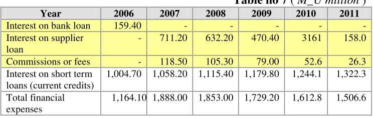
Table no 7 ( M_U million )

Year 2006 2007 2008 2009 2010 2011

Interest on bank loan 159.40 - - - - -

Interest on supplier loan

- 711.20 632.20 470.40 3161 158.0 Commissions or fees - 118.50 105.30 79.00 52.6 26.3 Interest on short term

loans (current credits)

1,004.70 1,058.20 1,115.40 1,179.80 1,244.1 1,322.3 Total financial

expenses

1,164.10 1,888.00 1,853.00 1,729.20 1,612.8 1,506.6

Because a large proportion of 2005’s interests expenses

come from bank loans, having a value of M_U 1,223,264 thousand, there results a current loans expenses of M_U 18.9 for each M_U 1,000

operating income and an estimation of interests' outlay on current

credits of M_U 15 for each M_U 1,000 revenue (estimation being used in previous table).

An important tool in the analysis and investigation process

is the company’s forecast expenses and income budget - detailed as

following:

Income and expenses budget

Table no 8 (M_U Million)

2006 2007 2008 2009 2010 2011

Total income, of that:

68,512.4 72,149.1 76,030.9 80,407.9 84,407.9 90,089.0 Operating

revenue

Total expenditure, of which:

64,338,3 68,096,5 70,649,6 73,352,1 76,284.0 79,052.0

Operating expenses

63,174.2 66,208.5 68,796.8 71,622.9 74,671.2 _77,545.4 a)Raw materials 30,508.3 31,642.2 32,833.4 34,133.7 35,733.0 36,775.1 b)Employees 7,804.4 8,038.7 8,284.6 8,553.3 8,806.9 9,098.9 c)Depreciation 952.9 1,522.7 1,522.7 1,522.7 1,522.7 1,522.7 Financial outlays 1,164.1 1,888.0 1,853.0 1,729.2 1,612.8 1,506.6 Gross operating

profit 4,174.1 4,052.6 5,381.3 7,055.8 8,123.9 11,037.0

o assuming a legal reserve percent of 5% and a fiscal charge

percent of 30% (higher than a regular current fiscal charge for the country having that M_U currency), the followings data are going to be obtained ( - all these values are chosen according to the necessity of checking/hedge an adverse fiscal policy in order to cover any unwanted exposures):

Table no 9 (M_U Million)

2006 2007 2008 2009 2010 2011

Legal reserve 208,7 202,6 269,1 352,8 406,2 551,9 Corporate tax 1,189.6 1,155.0 1,533.7 2,010.9 2,315.3 3,145.5 Net income after

taxes 2,775.8 2,695.0 3,578.6 4,692.1 5,402.4 7,339.6

Net cash benefit 3,728.7 4,217.7 5,101.3 6,214.8 6,925.1 8,862.3

Cash-flow from operating activities

4,892.8 6,105.7 6,954.3 7,944.0 8,537.9 10,368.9

Based upon the last notices, it can be observed an

increasingly positive value for the cash-flow.

The analysis is going to continue with a forecast for

balance sheet and its elements: Current assets

Characterized by:

• The participation of inventory

2005 36,238,664 / 6,249,368 = 5.78

2004 19,914,374 / 2,901,467 = 6.86

The tendency is downward. The forecast is using an assumption of stop-low level for 2006, followed by an yearly growth with 0.5 rotations for the next four years. This assumption is necessary for our process. All used data about 2005 year are recorded into the attached annexes.

• Receivable (including all regularized accounts)

2005 36,238,664 / 4,675,513 = 7.75

2004 19,914,374 / 1,757,396 = 11.3

an increasing ratio with one rotation per annum for the next four years is reliable.

• Cash account

The proportion of cash into current assets was:

2005 6.1%

2004 3.2%

The ratio has followed an uptrend, although its level is still unsatisfactory because otherwise it requires a percent of 30%. It is consider that 10% can be achieved and sufficient for a normal activity. The structure for the future current assets based on previous conclusions, is set in the next table:

Table no 10 (M_U Million)

2006 2007 2008 2009 2010 2011

Sales 66,976.90 70,546.90 74,357.00 78,654.10 82,941.50 88,157.50 Inventory 6.38

10,497.90 6.88 10,253.90 7.38 10,075.50 7.88 9,981.50 7.88 10,525.60 7.88 11,187.50 Receivable 7.75

8,642.20 8.75 8,062.50 9.75 7,626.40 10.75 7,316.60 10.75 7,795.30 10.75 8,200.70 Cash 1,914 2,747.5 3,540.3 4,324.5 5,496.3 6,785.9 Current

assets

21,054.10 21,063.90 21,242.20 21,622.60 23,817.40 26,174.10

Obligations

About their elements there should be observed the next features:

• Suppliers and creditors

2005 36,238,664 / 2,059,978 = 17.6

2004 19,914,374 /1,751,890 = 11.3

As it can be noticed, the rotation ratio is growing. Thus, the average length of credit is of 20 days. For an efficient use of financial resources it is necessary a reduced ratio and supposed an analysis starting at a normal ratio and finishing at a ratio equal to that of 2005.

• Other debts

2005 36,238,664 / 2,390,397 = 15.1

2004 19,914,374 / 1,149,519 = 17.3

The rotation ratio is important but it is known that a normal ratio requires a level of almost 8, according to 45 days. Related to this criteria the analyst should establish a reduction of ratio, and the overall debts are:

Table no 11 (M_U Million)

2006 2007 2008 2009 2010 2011

Suppliers 8 8,372.10 10 7,054.70 12 6,196.40 14 5,618.10 16 5,183.80 17 5,185.70 Other debts 12

There appears an opportunity for a link between the total obligations and the current assets, followed by a forecast evolution of company’s fixed plants.

C u r r e n t a s s e t s O b l i g a t i o n s 2 0 0 6 2 0 0 7 2 0 0 8 2 0 0 9 2 0 1 0 2 0 1 1 0 . 0

5 0 0 0 . 0 1 0 0 0 0 . 0 1 5 0 0 0 . 0 2 0 0 0 0 . 0 2 5 0 0 0 . 0 3 0 0 0 0 . 0

Figure no 11 – Current assets and commercial obligations

FIXED ASSETS

Table no 12 (M_U Million)

2006 2007 2008 2009 2010 2011

Fixed plants at residual value -existing at year beginning

65,556.10 64,603.20 69,945.69 69,174.78 68,990.17 68,921.06

-acquisitions - 6,865.20 751.8* 1,338.1* 1,453.6* 1,506.5*

-sales - - - -

Fixed plants at year end

65,556.10 71,468.40 70,697.49 70,512.88 70,443.77 70,427.56 Amortization 952.90 1,522.71 1,522.71 1,522.71 1,522.71 1,522.71 Net fixed

assets

6,4603.2 69,945.69 69,174.78 68,990.17 68,921.06 68,904.85 Possible new

tangible assets

6,865.20 - - - - -

Participation 500.00 500.00 500.00 500.00 500.00 500.00 Total 71,968.40 70,445.69 69,674.78 69,490.17 69,421.06 69,404.85

*The replacement investments should be equal to depreciation

As a result of previous calculus, it can be forecast the

probable history of Balance Sheet in case of financing by loans

(commercial and banking loans):

Table no 13 (M_U Million)

2006 2007 2008 2009 2010 2011

Current assets

21,054.10 21,063.90 21,242.20 21,622.60 23,817.40 26,174.10 Total assets 93,022.50 91,509.59 90,916.98 91,112.77 93,238.46 95,578.95 Equity 66,546.30 66,546.30 66,546.30 66,546.30 66,546.30 66,546.30 Reserve 1,409.70 1,608.00 1,869.00 2,297.60 2,692.30 3,270.00 Other funds 2,193.70 3,612.30 3,611.70 5,514.60 9,293,00 13,401.10 Net worth 70,149.70 71,766.60 72,455.60 74,358.50 78,531.60 83,217.40 Medium

term liabilities

5,925.20 5,266.70 3,950.00 2,633.30 1,316.60 -

Debts 13,953.50 12,933.60 11,916.20 11,236.20 11,108.20 11,062.90 Short term

liabilities

2,994.10 1,542.69 2,595.18 2,884.77 2,282.06 1,298.65 Liabilities

total

22,872.81 19,742.99 18,461.38 16,754.27 14,706.86 12,361.55 Net worth+

liabilities total

93,022.50 91,509.59 90,916.98 91,112.77 93,238.46 95,578.95

Main economic activity indicators

Using the previous data, it can be computed the influence

upon the fundamental indicators as following:

• Sales

Year 2005 2006 2007 2008 2009 2010 2011

Value (M_U mill.)

36,238.7 66,976.9 70,546.9 74,357.0 78,654.1 82,941.5 88,157.5

The favorable trend for sales, is based both on modernizing

investment and diversification of company’s activity.

• Current account = Current assets / Current liabilities

Year 2005 2006 2007 2008 2009 2010 2011

Index 1.13 1.24 1.46 1.46 1.53 1.78 2.12

The indicator presents the overall capacity of meeting

short-term obligations using cash, receivable and inventory. The evolution has a positive effect upon the operating cash-flow.

• Quick ratio = Current assets-inventory / Short term liabilities

Year 2005 2006 2007 2008 2009 2010 2011

Index 0.52 0.62 0.75 0.77 0.82 0.99 1.21

Related to previous information, this indicator confirms

both the lack of default risk and the favorable trend obtained by a higher level than the critic one.

Q u i c k r a t i o C u r r e n t a c c o u n t

2 0 0 5 2 0 0 6 2 0 0 7 2 0 0 8 2 0 0 9 2 0 1 0 2 0 1 1

0 0 . 5 1 1 . 5 2 2 . 5 3 3 . 5

• Gross return on net assets = Gross Profit *100 / Assets

Year 2005 2006 2007 2008 2009 2010 2011

Percent 0.59 4.49 4.43 5.92 7.74 8.71 11.55

It is obvious an approach of managerial team in generating

profit by an increased participation of assets to product process. It is necessary a correlation with the other return ratio.

• Return on shareholders’ equity = Net Profit*100 / Net

Wealth

Year 2005 2006 2007 2008 2009 2010 2011

Percent 0.34 3.96 3.76 4.94 6.31 6.88 8.82

It resumes the efficiency of investment use for

shareholders’ equity. The uptrend tendency suggests a better guaranty for lender or investor.

• Gross profit ratio = Gross Profit *100 / Sales

Year 2005 2006 2007 2008 2009 2010 2011

Percent 1.31 6.23 5.74 7.24 8.97 9.79 12.52

The better the return the more attractive the company. This reality is the result of a lower production cost per products and an active marketing policy, all these being the effect of innovation and new plant implementation.

• Patrimonial solvability = Net worth*100 / Assets

Year 2005 2006 2007 2008 2009 2010 2011

Percent 87.2 75.4 78.4 79.7 81.6 84.2 87.1

It reflects the proportion of shareholders’ equity into total

assets, which means a better capacity of financial autonomy along these years.

• Gearing ratio = Liabilities*100 / Shareholders’ equity

Year 2005 2006 2007 2008 2009 2010 2011

Percent 14.6 32.6 27.5 25.5 22.5 18.7 14.9

The level of financial independence as previous ratio has

shown, is going to reach a favorable trend with direct implications upon the company’s behavior in borrowing. It is said that there is an active policy for financing by internal sources.

• Receivable collection period = Trade receivable*365 / Sales

Year 2005 2006 2007 2008 2009 2010 2011

Days 42.9 47.1 41.7 37.4 33.9 33.9 33.9

The credit policy toward its customers is going to know

favorable tendency. In this way, the necessity of short term borrowed money is lower. It is the result of a more active juridical department.

• Credit repayment period = Accounts trade payable*365 /

Sales

Year 2005 2006 2007 2008 2009 2010 2011

Days 98.8 124.6 100.6 90.51 77.7 64.7 51.1

Although it reaches high values at the beginning, starting

with 2008 it arrives at low levels. This movement does a good “impression” over the creditors’ behavior.

Year 2005 2006 2007 2008 2009 2010 2011

Ratio (mill. M_U)

22.2 41.1 43.3 45.6 48.2 50.8 54.1

By this indicator it is measured the value of production per

employed labor force. Thus, the results show an increased participation of workers that has come from investment process.

• Interest coverage ratio = EBIT / Interest

Year 2005 2006 2007 2008 2009 2010 2011

Indicator 1,2 4,4 3,0 3,8 4,9 5,8 8,0

The usual value of this indicator is around 3. There is an uptrend due to a stronger competitive production on the market due to investments.

Using the previous ratio analysis, there are concluded the

followings:

1. The company will be capable to meet its current liabilities both with and without use of inventory. The inventory-based ratios are into the acceptance borders.

2. Profitability ratio is still going to be below the optimal level for the

economy, but compared to 2005 year, they have known a certain improvement.

3. Solvability is higher than the 30 per cent minimum accepted

border, so there can be a great confidence of lenders and suppliers into this kind of managerial policy.

4. By using external funds, we are witness to the improvement of

financial autonomy that has a better influence upon the return of shareholders’ equity.

5. The income from interest and from favorable exchange rates is

going to follow the trend of operating revenue.

6. Debtor collection period and creditor payment period are the same

for all kind of investment financing and go toward the regular level. On medium term there cannot appear important changes into the relations with suppliers, customers and lenders.

7.

levels in this appraisal.

BONDS ISSUES

An alternative to the banking/supplier loan is the bond

• Accountancy analysis for year 2005 in previous “chapters”;

• Forecast of income for 2006 till 2011 from last

“chapter”;

• Forecast of operating expenses;

• Disclosure of current assets and obligations due to

suppliers from 2006 up to 2011;

• Statement of forecast fixed assets.

The economic analysis upon the company for year 2005,

together with the investment revenue, have as effect/influence a ranking into a low risk level. Thus, there is going to be used a discount risk rate of 25 percent, and the result for issued interest rate is the formula:

Rd = (1+Rp)(1+Rr)-1

where Rp means the Market Interest Rate for FRG deposits Rr means the FRG Discount Risk Rate

and being required an yield of 12% for FRG deposits (the higher expectation, the higher yield), there are obtained:

Rd = 14%

Now, there should be considered the assumptions that were

used as the starting base for previous commercial loan analysis:

a. decrease in the financing by internal funds;

b. increase of gearing;

c. a low net working capital;

d. a low working capital covering for assets;

e. an increased number of participation for assets;

f. decrease in the difference between current assets and short

term liabilities ;

g. decrease in current assets covered by net worth.

So, the bond issue can be described:

Issue value is equal to the face value of FRG 14,600,000 (the final value of FRG 14,606,811 was approximated in order to reduce the difficulty level of calculus);

Coupon of 14%;

Borrowing period is 6 years;

Placement is done by a department of issuer; Interest rate is paid yearly;

Redeem is going to be done at the end of the sixth year and to be paid by a single settlement;

Insurance commission is 2% of the outstanding remained payment value, payable yearly.

All these elements should be considered as reliable

expenses together with their implication about balance sheet statement and economic indexes.

Yearly outflows’ situation comes to be:

Insurance commission

Table no 14

Year 2006 2007 2008 2009 2010 2011

Value FRG 292,000 292,000 292,000 292,000 292,000 292,000 Value M_U mill. 137.24 137.24 137.24 137.24 137.24 137.24

Repayment of loans

Table no 15

Year 2006 2007 2008 2009 2010 2011

Value FRG 0 0 0 0 0 14,600,000

Value mill. M_U 0 0 0 0 0 6862.00

Interest rates

Table no 16

Year 2006 2007 2008 2009 2010 2011

Value FRG 2,044,000 2,044,000 2,044,000 2,044,000 2,044,000 2,044,000 Value mill.

M_U

960.68 960.68 960.68 960.68 960.68 960.68

- using the same value for the short-term loans’ interest rate, it can be obtained:

Table no 17

Year 2006 2007 2008 2009 2010 2011

Short-term interest rate

1,004.70 1,058.20 1,115.40 1,179.80 1,244.10 1,322.30 Total financial

expenses 2,102.62 2,156.12 2,213.32 2,277.72 2,342.02 2,420.22

Based on the previous results, there is not hard to forecast

the dynamic economic activity:

Income and expenses budget

Table no 18 (M_U Million)

2006 2007 2008 2009 2010 2011

Total revenue, of which:

68,512.4 72,149.1 76,030.9 80,407.9 84,407.9 90,089.0 Operating

income

66,976.9 70,546.9 74,357.0 78,654.1 82,941.5 88,157.5 Financial income 1,535.5 1,602.2 1,673.5 1,753.8 1,834.0 1,931.5 Total expenses,

of which:

65,276.8 68,364.6 71,010.1 73,900.6 77,013.2 79,965.6 Operating

outlays 63,174.2 66,208.5 68,796.8 71,622.9 74,671.2 77,545.4 a)Raw materials 30,508.2 31,642.2 32,832.5 34,133.7 35,370.2 36,775.1 b)Employees’

wages