A Parallelized Matrix Multiplication Implementation of Neural Network for Collision Free Robot Path Planning

A Parallelized Matrix-Multiplication Implementation of

Neural Network for Collision Free Robot Path Planning

Abhishek Kumar

Department of Computer Engineering Indian Institute of Technology – (BHU)

Varanasi, India

Ravi Bhushan Mishra

Department of Computer Engineering Indian Institute of Technology - (BHU)

Varanasi, India

ABSTRACT

This paper covers the problem of Collision Free Path Planning for an autonomous robot and proposes a solution to it through the Back Propagation Neural Network. The solution is transformed into a composition of matrix-multiplication operations, which is a classic example of problems that can be efficiently parallelized. This paper finally proposes a parallel implementation of this matrix-multiplication method which, in itself, encapsulates the neural network that implements the collision free path planning for an autonomous robot.

General Terms

Robot Path Planning, Back Propagation Neural Networks, Parallel Neural Networks

Keywords

Robot Path Planning, Back Propagation Neural Networks, Parallelism, Matrix-Multiplication

1.

INTRODUCTION

Collision free path planning of an autonomous robot is a classic problem in the realm of robotics. It is mainly concerned with equipping the robot with a technology that allows it to get from a source to a destination safely, while avoiding any obstacles in its path, without any external aid.

As highlighted in [3], the problem of collision free path planning of an autonomous robot can be decomposed into two sub-problems -

1. Findspace Problem 2. Findpath Problem

The Findspace problem deals with mapping the problem space, in this case, the physical structure of the area that contains the robot's current position, its destination and the probable intermediate locations, with a way to specify the obstacles.

The Findspace problem involves scanning the area in the vicinity of the robot to ascertain the locations of various obstacles that might obstruct the robot's path from the source to the destination. This is usually done by a sensor mounted on the robot which more generally uses some kind of waves and their reflections from nearby obstacles to form a map of the surrounding area (much like sonar). There can be alternative means for space mapping which may involve capturing an image of the surrounding region to find the locations of obstacles.

The Findpath problem is finding a safe, collision free route

from the source to the destination. It is involved with using the information obtained through the solution of the Findspace problem to find a trajectory for the robot to follow, which will ensure a collision free motion of the robot from the source to destination.

Various approaches to the Findpath problem has been discussed and implemented over time, highlighting the various approaches that can be used to solve the problem, although each such method has its own advantages and shortcomings based on accuracy, efficiency(time) and the difficulty of implementation.

As discussed in [4] Genetic Algorithm and Ant Colony Optimization are the two algorithms that can be used to solve the Findpath problem efficiently and accurately.

The Genetic Algorithm for solving the Findpath problem involves mutating the genes (which correspond to intermediate points of a path) to form new set of chromosomes (collection of genes that specify a solution), evaluating the fitness of the chromosomes (using some kind of fitness function) and taking the fitter chromosomes to the next generation while eliminating the less fitter ones. The Ant Colony Optimization approach to the Findpath problem performs a number of iterations to update the paths and associate with them a degree of goodness (pheromones).

The Neural Network approach has been used in this paper to solve the Findpath problem. A Neural Network is a collection of several computing units – neurons, connected in a graph topology through weighted connections (edges). The Neural Network approach to solve the Findpath problem can be broadly classified into two categories -

1. Supervised Neural Network 2. Unsupervised Neural Network

The Unsupervised learning methodology for neural networks does not have a pre-classified set of input – output patterns to train the network and instead use the Hebbian learning rule to update the weights.

2.

ORGANIZATION OF THE PAPER

Section 1 of this paper describes the general problem of Collision Free Path Planning of Autonomous Robot. Section 3 gives a brief overview of some research papers that propose various solutions to the path planning problem. Section 4 describes accurately our problem space and our set up towards its solution. Section 5 describes the theoretical aspect of our implementation and the methodology involved in solving the Findpath problem in detail. Section 6 covers an overview of the implementation details and results. Section 7 covers the conclusion and the future wok possible followed by acknowledgment and references in section 8 and 9 respectively.

3.

RELATED WORK AND RESOURCES

[1] proposes a method of path planning based on neural network and genetic algorithm. The neural network model is used to construct the workspace for a robot and this model is used to establish the relationship between a collision free path and the output of the model. Then the two-dimensional coding for the path via-points was converted to one-dimensional and the fitness of both the collision avoidance path and the shortest distance are integrated into a fitness function to be used in the Genetic Algorithm.

[2] specifically addresses the problem of collision free path planning in an autonomous space robot. The paper uses a back-propagation neural network and three layers – input layer with 2 neurons, hidden layer with 3 neurons and output layer with 2 neurons to implement a solution. The activation function for the hidden layer is sigmoid function and that for output layer is the identity function.

[4] uses genetic algorithm and ant colony optimization to provide a solution to the general path planning problem as well as discuss the benefits and the limitations associated with each of them.

[3] again deals with path planning and intelligent control of an autonomous robot which should move safely in partially structured environment. However, it addresses both the problems – Findspace problem and Findpath problem and uses two neural networks – one to map the space and hence solve the Findspace problem and the other to deal with the construction of a collision free path through the partially structured space to avoid the nearest obstacles.

4.

THE PROBLEM SETUP

The space through which a robot has to reach its destination is envisioned as an N x M (N being number of rows and M number of columns) grid of 0.1 unit x 0.1 unit squares. Each of the squares is marked with 1 – specifying the location of an obstacle over that square, or 0 – specifying the lack of it.

This grid map is imposed over the space to facilitate a quantitative view of the problem space.

Moving on to our neural network, the neural network has three layers -

1. Input layer – Input layer has 2 neurons – to be fed the 2 co-ordinates – row co-ordinate and column co-ordinate – of the current position of robot.

2. Hidden Layer – Experiments were carried out with a

variable number of neurons in the hidden layer – from 3 to 100 to 1000 – and a good result for medium sized input was obtained for 1000 neurons in the hidden layer.

3. Output Layer – It has two output neurons, to output the row and column co-ordinate where the robot should move to in the next step for the input row and column co-ordinate.

In addition to the above mentioned neurons, there are two biases – one each in the input and the hidden layer, each fed with an input of 1.

Two sets of weights can be identified for our setup – W(i,j)(1) ,

which is the weight of synapse between the ith neuron in the input layer and the jthin the hidden layer and W(i,j)

(2),

the weight of the synapse between the ith neuron in the hidden layer and the jthneuron in the output layer.

The weights are initially randomly initialized with a small value between 0.001 to 0.1 and updated thorough multiple training passes.

The learning rate was chosen to be 0.25.

The operation of the network involves two phase -

1. Training phase, over which a number of (input, output) patterns are presented to the network and the weights are appropriately updated by comparing the obtained output with the expected output.

2. Operation phase, in which an input is presented to the network and the obtained output is used to decide the next step of motion.

The number of training patterns varies with the complexity of the problem space and the accuracy desired.

5.

THE PROPOSED MODEL

5.1

The Back-Propagation Algorithm

First, the error function is defined as the function that measures the squared difference between the expected and the obtained output in each iteration. The back-propagation algorithm aims at finding the optimal combination of weights of the synapse that minimizes this error function. For this we follow a method of gradient decent. The weight of a synapse is moved in the direction that aims to minimize the error. More formally, the weight of a synapse is shifted in a direction opposite to the gradient of the error with respect to the weight.

The ability of being able to calculate the gradient of the error function at each step requires the error function, and hence the activation function for each of the neuron ( in the hidden and the output layer ) to be differentiable. Let the activation function be f for both – the hidden and the output neurons.

Let the input to the two input neurons are x and y respectively and 1 to the bias, which they pass on as their output.

A

j (1)

= Σ W

(i,j)

(1)

. O

i

where, Oi is the output from the ithinput neuron, W(i,j)(1) is the

weight between the ith _{input neuron and the j}th_{hidden neuron}

and i varies in summation from 1 to 3 (signifying 3 input neurons including the bias).

If the activation function for the hidden neurons is f, then the output from the jth hidden neuron is

O

j

(1)

= f( A

j

(1)

)

Similarly, The activation for the jthoutput neuron as such can be given as,

A

j (2)

= Σ W

(i,j)

(2)

. O

i (1)

where, Oi(1) is the output from the ithhidden neuron, W(i,j)(2) is

the weight between the ith hidden neuron and the jthoutput neuron and i varies in summation from 1 to k ( signifying k hidden neurons including the bias ).

If the activation function for the output neurons is f, then the output from the jth output neuron is

O

j

(2)

= f( A

j

(2)

)

During the operation phase, the collection of all outputs (from the 1st and the 2nd output neuron) specifies the next step for the robot.

During the training phase, if the expected output from the jth output neuron is Pj, then the error from the jth neuron is

calculated as

E

j

=0.5 .( O

j

(2 )

- P

j

)

2

As such, the overall error is the collection of errors from all outputs and is given as

E=Σ 0.5 .( O

j(2 )

- P

j

)

2

where summation is calculated for j from 1 to 2 (due to two output neurons).

The steps discussed so far constitute the forward pass of the back-propagation algorithm.

During the error back-propagation phase, for each weighted synapse with weight w, the gradient with respect to the weight is calculated and the weight is moved in the direction opposite to this gradient. Mathematically, after the tth iteration, the weight Wtof any synapse, with weight Wt- 1 before the

iteration, is given as

W

t

=W

t – 1

–η . ∂E / ∂W

t – 1

where, η is the learning rate, E is the total error as defined above and ∂ E / ∂ Wi – 1 is the partial derivative of E with

respect to Wi – 1.

Applying the above formula to the weights between the hidden and the output layer gives

W

(i,j)(2)t

=W

(i,j)(2)t – 1

–η . δ

j(2)

. O

i(1)

...(1)

where symbols have predefined meanings and,

δ

j(2)

= ∂O

j(2 )

/ ∂A

j(2) .

(O

j(2 )

-P

j

) …(2)

where symbols have predefined meanings.

Similarly for the weights between the input and the hidden layer we have

W

(i,j) (1)

t

=W

(i,j) (1)

t – 1

–η . δ

j (1)

. O

i

...(3)

where symbols have predefined meanings and,

δ

j (1)

= ∂O

j

(1 )

/ ∂A

j

(1)

.

Σ(W

(j,q) (2)

_.δ

j (2)

) ...(4)

where symbols have predefined meanings and the summation is carried for q varying from 1 to 2 (signifying two output neurons).

The weights are updated during the back-propagation step as explained. This process continues for various training iterations after which the network becomes sufficiently trained for operations.

During the operation phase only the forward pass is executed to obtain the outputs.

5.2

Parallel Matrix Multiplication

Implementation of Back-Propagation

Algorithm

The computations described previously can be gathered into a few operations of matrix-multiplication. Matrix-multiplication being a classical problem that can be parallelized, the reduction of all the above described computations into one or more matrix-multiplication provides an opportunity to parallelize the overall neural network operations. Before describing the reduction of computations into a few operations of matrix-multiplication, a few matrices need to be defined that will be used in the discussion that follows.

Ô is defined as a 1 x 3 matrix (a vector) of the outputs of the input neurons (including bias)

Ô = O

1,

O

2

, O

3

Similarly, Ô(1) _{is defined as the 1 x k matrix of the outputs}

from the hidden neurons ( including the bias )

Ô

(1)

= O

1 (1)

,

O

2

(1)

_{, … , O}

k (1)

∂O

1(1 )

/∂A

1(1)

0 0 … 0

D1= 0 ∂O

2

(1)

_/∂A

2

(1)

_{0 … 0}

… … … … … …

0 0 0 … ∂O

k-1(1)

/∂A

k-1(1)

where symbols have the same meanings as defined previously and k - 1 is the number of hidden neurons excluding the bias.

Similarly is defined D2, a 2 x 2 matrix, as

D2 = ∂O

1

(2 )

_/∂A

1

(2)

0

0 ∂O

2

(2)

_/∂A

2

(2)

where the symbols have the same meanings as defined previously.

Another 2 x 1 matrix E is defined as

E = O

1

(2 )

-P

1

O

2

(2 )

-P

2

with symbols holding the same meanings as before.

The weight matrix Ŵ1 is a 3 x k matrix for weights between

the input and the hidden layer, such that ŵ1( i, j ) is the weight

of the synapse from the ith input neuron to the jthhidden neuron.

Similarly is defined the k x 2 matrix Ŵ2 for the weights

between the hidden and the output neuron.

W1 is the 3 x (k – 1) weight matrix formed from the matrix

Ŵ1 by removing the column corresponding to the bias in the

hidden layer.

Similarly is formed the matrix W2 from Ŵ2.

After having all the terminologies in place, the operations defined previously are transformed and grouped together as matrix-multiplication operations.

Beginning with the feed-forward operation, the outputs from the hidden neurons can be collected into a 1 x (k – 1) matrix O(1) _{(excluding the bias) which is given as}

O

(1)

= f( Ô x Ŵ

1

)

where f is the activation function to be applied on each element of the obtained product matrix.

Similarly, the outputs from the output layer can be gathered into a 1 x 2 matrix O(2) as

O

(2)

= f( Ô

(1)

x Ŵ

2

)

Now moving towards the back-propagation the following reductions are needed as cited below.

Equation (2) for all j's can be transformed into

δ

(2)

= D

2

x E

Similarly, equation (4) for all j and q can be transformed into

δ

(1)

= D

1

x W

2

x δ

(2)

As such equation 1 for all i, j becomes,

Ŵ

2(t) (T)

_=Ŵ

2(t – 1)

(T)

_{–η . δ}

(2)

. Ô

(1)

where, (T) stands for the transpose of the matrix.

Similarly, the updating of weights between the input and the hidden layer is done for all i,j by,

Ŵ

1(t)

(T)

_{= Ŵ}

1(t – 1)

(T)

_{–η . δ}

(1)

. Ô

which is the reduced form of the equation (3).

To sum up, each iteration during training requires four matrix-multiplications and two matrix subtraction, whereas during the operation phase only two matrix-multiplications are required.

6.

IMPLEMENTATION AND RESULTS

The methodology discussed above was implemented in C++. The OpenMpapi was used for implementing thread level parallelism.

The overall algorithm was broken down into steps of matrix-multiplication and these matrix-multiplications were parallelized using the directives and constructs of OpenMp.

To begin with finer-level details – the neural network was constructed and tested with 3 hidden neurons, 100 hidden neurons and 1000 hidden neurons. The best result was obtained with 1000 hidden neurons. A neural network with 1000 hidden neurons could deal with versatile problem scenarios for small to medium scale problem space and yet provide a sufficiently accurate result. The activation function f

was chosen to be the identity function ( f(x) = x ). Hence the partial derivative, ∂f/∂x = 1.

The parallel program was tested on a uniprocessor system, a two-processor system and a four processor system and a near optimal speed-up was obtained. A twp processor system yielded a speed-up about 1.9, while for a four processor system it was about 3.7.

[image:5.595.318.544.71.299.2]

Fig 1: Change in the run-time with change in the number of processors

The change in the run-time of the program with the change in the number of processors is graphically depicted above.

As can be seen, the speed up obtained is proportional ( and very nearly equal ) to the number of processors. For a medium sized input, the program took 18 ms to execute on a uni- processor system. While for the same input it took 9 ms on a 2-processor system and 5 ms on a 4-processor system.

The overall variation of the run-time (r) on an input with the number of processors (p) can be approximately represented as

rp = k

for some constant k.

Considering the operation of the neural network, the implemented neural network was experimented with various problem and space and in each of those the robot could safely avoid any obstacles and reach the destination using a sufficiently good path. In each of the cases, the robot would stop moving when it has reached close enough to the destination.

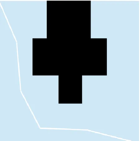
[image:5.595.55.280.76.306.2]

For instance, when the network was trained on a square grid with the area in the vicinity of the center of the square filled with obstacles and the robot released from the top left corner with the destination being the bottom right corner, the robot could safely avoid the obstacles and reach the desired destination as depicted below. The constructed path in this case consists of four intermediate points between the starting and the destination point.

Fig 2: Trajectory of the robot for an obstacle-filled problem space

7.

CONCLUSION AND FUTURE WORK

This paper presented a neural network approach to the problem of collision free path-planning of an autonomous robot, and thereafter transformed it into a sequence of matrix-multiplications which were parallelized on a multiprocessor system. Thread level parallelism was used for parallelization. The speed-up obtained was near-optimal. The robot was successfully able to move from a starting source position to a destination while avoiding obstacles.

As a future endeavor, further research can be made to specify and outline the architectural design so as to achieve a higher degree of parallelism as well as make the program even more efficient. Such a design shall remove the limitations that come with implementing parallelism at the application level such as context switch overheads, synchronization etc.

8.

ACKNOWLEDGMENT

We are thankful to all who helped in this project’s execution.

9.

REFERENCES

[1] DU Xin 1, CHEN Hua-hua 2, GU Wei-kang1/ Neural network and genetic algorithm based global path planning in a static environment, (1 Department of Information Science and Electronics Engineering, Zhejiang University, Hangzhou 310027, China)(2 School of Communication Engineering, Hangzhou Dianzi University, Hangzhou 310018, China)

[2] Youssef Bassil / Neural Network Model for Path-Planning Of Robotic Rover Systems, International Journal of Science and Technology (IJST), E-ISSN: 2224-3577, Vol. 2, No. 2, February, 2012

Systems, Volume 1 Number 1 (2004), ISSN 1729-8806.

[4] Kyung Min Han, Collision Free Path Planning Algorithms for Robot Navigation Problems, A Thesis presented to the faculty of the Graduate School University of Missouri-Columbia, 2007